AMBA APB · Module 14
APB Latency Anatomy
Decomposing the latency of a single APB transfer cycle by cycle — the one SETUP cycle, the one-or-more ACCESS cycles, and exactly where the wait states land. The 2 + N cost model every throughput, utilisation, and system-impact argument is built on.
You have learned how APB works — phases, handshakes, errors, bridges. This module asks a different question: how much does it cost? And every cost answer — throughput, utilisation, the software-visible price of a register access — is built on one foundation: the cycle-by-cycle latency of a single transfer. The single idea to carry: an APB transfer's latency decomposes cleanly into exactly one SETUP cycle, plus one ACCESS cycle, plus N wait cycles — 2 + N clocks — and nothing else. There is no pipelining to amortise, no overlap to exploit; the latency is a simple, exact sum you can count off a waveform. Learn to decompose it precisely here, and the throughput math, the utilisation curves, and the DMA-versus-CPU arguments in the rest of the module become arithmetic.
1. Problem statement
The problem is assigning an exact, decomposed cycle cost to one APB transfer — not a hand-wave like "a couple of cycles," but a precise account of where every clock goes, so the cost can be reasoned about, compared, and budgeted.
Performance work starts with an honest unit cost. For APB that unit is a single read or write, and its latency has to be pinned down to the cycle because everything downstream multiplies it:
- The fixed floor is two cycles. Every APB transfer is two-phase: a SETUP cycle (
PSELhigh,PENABLElow) and an ACCESS cycle (PENABLEhigh). Even an instantly-ready slave costs two clocks — there is no one-cycle APB transfer. That floor is the irreducible cost of the protocol's structure. - Wait states add exactly, and only, to ACCESS. A slow slave extends the ACCESS phase by holding
PREADYlow; each held cycle is one extra clock. SETUP is never extended. So the total is1 (SETUP) + 1 (ACCESS) + N (waits) = 2 + N, whereNis the number ofPREADY-low cycles. - There is nothing else in the sum. No arbitration latency baked into the transfer (APB has no in-transfer arbitration), no pipeline fill, no turnaround bubble within a single transfer. The decomposition is complete at
2 + N— which is precisely what makes APB's cost so easy to reason about, and what later chapters lean on.
So the job is to take any APB transfer and read its latency as the exact sum 2 + N, knowing which phase each clock belongs to — the unit cost the whole performance module is denominated in.
2. Why previous knowledge is insufficient
You already know the mechanics — the setup phase, the access phase, how PREADY extends ACCESS. What you have not done is turn that mechanism into a number:
- You learned the phases as behaviour, not as cost. Every prior chapter described what happens in SETUP and ACCESS. This module reads those same phases as clocks spent. The shift is from "the access completes when
PREADYis high" to "this access cost2 + Ncycles, of whichNwere wait states" — the mechanism re-expressed as a latency budget. - Wait states were a correctness topic; here they are the variable cost. Module 8 treated
PREADY=0as flow control to implement correctly. From a performance seat,N(the wait count) is the knob: a zero-wait peripheral costs 2 cycles, a 10-wait flash read costs 12. The same signal you learned to drive is now the dominant term in the cost. - Single-transfer cost is the atom of all the math. Throughput, utilisation, and access cost are all aggregates of this one number. You cannot compute transfers-per-second or bus utilisation without first knowing, exactly, what one transfer costs — so the decomposition is the prerequisite the rest of the module silently assumes.
So the model to add is the budget view: each phase as a line item in clocks, summing to 2 + N, that becomes the building block for every aggregate cost.
3. Mental model
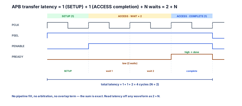
The model: an APB transfer is a two-stroke engine with optional stall cycles. Stroke one is SETUP (always one cycle), stroke two is ACCESS (always one cycle of useful completion), and if the slave isn't ready, the engine idles in the ACCESS stroke for N cycles before firing. Count the strokes and the idles and you have the exact latency: 1 + 1 + N. The engine never skips a stroke and never overlaps two transfers' strokes — so the count is always honest.
Three refinements make it precise:
- SETUP is a fixed one-cycle line item. It is the cycle the manager asserts
PSELand presents address/control withPENABLElow. It is never extended and never skipped — a constant1in every transfer's budget. - ACCESS is one useful cycle plus the wait tail. The manager raises
PENABLEand samplesPREADYeach cycle. The cyclePREADYis finally high is the one useful ACCESS cycle (the completion); every earlierPREADY-low cycle in ACCESS is a wait. So ACCESS costs1 + N, andNis read directly as the number ofPREADY-low cycles before completion. - The total has no hidden terms. Latency
= 1 (SETUP) + 1 (ACCESS completion) + N (waits) = 2 + N. A best-case zero-wait transfer is exactly 2 cycles; there is no faster APB transfer. This exactness — no pipeline, no amortisation, no arbitration baked in — is the property the whole performance module exploits.
4. Real SoC implementation
In practice the decomposition is something you measure — in simulation or with a hardware performance counter — by timestamping the phases of each transfer. A small monitor that counts SETUP, wait, and completion cycles turns the model into hard numbers.
// A latency monitor: decompose each APB transfer into 2 + N cycles.
// Counts the wait states (N) and the total latency, per transfer.
logic [15:0] wait_cnt, latency_cnt;
logic        in_xfer;

always_ff @(posedge pclk or negedge presetn) begin
  if (!presetn) begin
    in_xfer <= 1'b0; wait_cnt <= '0; latency_cnt <= '0;
  end else begin
    // SETUP cycle: PSEL high, PENABLE low -> a transfer begins (cost = 1).
    if (psel && !penable) begin
      in_xfer     <= 1'b1;
      latency_cnt <= 16'd1;          // the fixed SETUP cycle
      wait_cnt    <= 16'd0;
    end else if (in_xfer) begin
      latency_cnt <= latency_cnt + 1'b1;             // every ACCESS cycle counts
      if (penable && !pready) wait_cnt <= wait_cnt + 1'b1;  // a PREADY-low wait
      if (penable && pready) begin                   // completion: transfer done
        in_xfer <= 1'b0;
        // latency_cnt now holds 2 + N ; wait_cnt holds N. Sample them here.
        // assert: latency_cnt == 2 + wait_cnt  (the decomposition is exact)
      end
    end
  end
end
Two facts make this the right way to anatomise latency. First, the wait count N is the only variable — SETUP is always 1 and the completion ACCESS cycle is always 1, so latency = 2 + N holds by construction, and a monitor only needs to count PREADY-low cycles to know the whole budget. Second, measuring per-transfer N is what feeds the aggregates: histogramming N across a workload gives the average transfer cost that throughput and utilisation are computed from, and the worst-case N (a slow flash or CDC peripheral) is what bounds the software-visible access cost. The anatomy is not academic — it is the instrument you point at a real workload to get the numbers the rest of the module needs.
5. Engineering tradeoffs
The latency budget is fixed in structure (2 + N) but the value of N — and what you do about it — is where the engineering lives.
| Contributor | Cycles | Fixed or variable? | How to reduce it |
|---|---|---|---|
| SETUP phase | 1 | Fixed (always) | Cannot — structural to the protocol |
| ACCESS completion | 1 | Fixed (always) | Cannot — the one useful cycle |
Wait states (N) | N | Variable (per slave/access) | Make the peripheral single-cycle; register data ahead; avoid CDC on the hot path |
| Best-case transfer | 2 | Floor | This is the minimum — no faster APB transfer exists |
| Slow-peripheral transfer | 2 + N (N large) | Dominated by N | A flash/CDC read can be 10+; this dominates the cost |
The throughline: two of the three line items are immovable, so all latency optimisation is wait-state (N) reduction. A peripheral that genuinely answers in one cycle hits the 2-cycle floor; one behind a slow memory or a clock-crossing pays a large N that swamps the fixed cost. Knowing the decomposition tells you exactly where to spend effort — never on SETUP/ACCESS (you can't), always on N (you sometimes can).
6. Common RTL mistakes
7. Debugging scenario
The signature latency bug is not a functional failure but a performance surprise: a peripheral access that costs far more cycles than budgeted, traced to an unexpectedly large N — and the anatomy is exactly the tool that localises it.
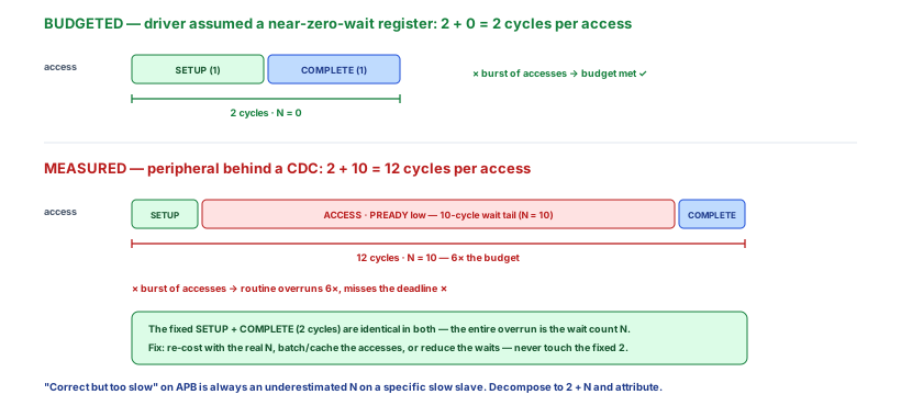
- Observed symptom: a driver routine that was budgeted at, say, 200 cycles for a burst of register accesses is measured at 1500 — a 7× overrun — and the system misses a real-time deadline. Functionally everything is correct; it is purely too slow.
- Waveform clue: decomposing the transfers on a trace shows the SETUP and completion cycles are exactly 1 each as expected, but the ACCESS phase of one particular peripheral's transfers is stretched —
PREADYstays low for 10+ cycles per access. The2 + Nbudget is being blown entirely by a largeNon one slave, not by anything in the bus or the other peripherals. - Root cause: that peripheral sits behind a clock-domain crossing (or a slow flash), so every access pays a long synchroniser/access latency as wait states. The driver was written assuming a near-zero-wait register, so its cycle budget used
N≈0when the realNis large — a costing error rooted in not knowing the per-access wait count. - Correct RTL: there may be nothing to "fix" in the RTL — the wait states are legitimate for a slow source. The fix is in the budget and the access pattern: re-cost the routine with the measured
N, and reduce the number of accesses to that slow peripheral (batch, cache the value, or move it off the hot path), or — if the latency is intrinsic and unacceptable — redesign the peripheral to register its data ahead so it answers in fewer waits. Where the waits were spurious (a needless CDC, an over-conservative ready), reducingNin the slave is the real fix. - Verification assertion: assert the decomposition holds so the monitor's numbers are trustworthy —
assert property (@(posedge pclk) disable iff(!presetn) (psel && penable && pready) |-> (latency_cnt == 2 + wait_cnt));— and add a performance assertion/coverpoint that flags any transfer whoseNexceeds the budgeted maximum for that address region, so a costing surprise trips in regression rather than in the lab. - Debug habit: when something is "correct but too slow" on APB, decompose the transfers into
2 + Nand look atNper peripheral. The fixed2is never the problem; a blown budget is always an underestimated wait count on a specific slow slave. MeasureN, attribute it to the peripheral, and decide between re-costing, reducing accesses, or reducing the waits — but start from the anatomy, not from guessing.
8. Verification perspective
Latency is a measured, not asserted, property, so the verification job is to make the measurement trustworthy and to catch costing surprises before silicon — performance regression alongside functional regression.
- Assert the decomposition is exact. Bind a property that every completed transfer satisfies
latency == 2 + N(whereNis the countedPREADY-low cycles). This is not a protocol check — it validates that your latency monitor is counting correctly, so the numbers feeding throughput and utilisation are sound. A miscounting monitor produces confident, wrong performance data. - Cover the wait-count distribution, not just functionality. Functional coverage should histogram
Nper address region: that zero-wait, one-wait, and the worst-case large-Naccesses were all seen. A suite that only ever exercises fast registers reports great functional coverage while never measuring the slow-peripheral latency that dominates the real cost — the performance hole hides behind functional green. - Add performance assertions with a budget. For latency-critical regions, assert that
Nnever exceeds the budgeted maximum (assert (... |-> wait_cnt <= MAX_N_for_region)), so an unexpectedly slow access — a new CDC, an over-conservative ready, a flash on the hot path — trips in regression. This turns "correct but too slow" from a lab surprise into a caught failure, which is the entire point of anatomising latency early.
The point: verify that the latency decomposition is measured correctly (2 + N holds), cover the wait-count distribution per region, and assert per-region wait budgets — so performance is regressed, not discovered.
9. Interview discussion
"What's the latency of an APB transfer?" sounds trivial and is actually a precision filter: the weak answer is "two or three cycles," the strong answer is the exact decomposition and why it has no hidden terms.
State it exactly: an APB transfer costs 2 + N cycles — one SETUP cycle, one ACCESS completion cycle, and N wait-state cycles where N is the number of PREADY-low cycles in the ACCESS phase. Then deliver the depth: the floor is two cycles (no one-cycle APB transfer exists, because the two-phase structure is mandatory even for an always-ready slave); wait states add only to ACCESS, one clock each (SETUP is never extended); and there are no other terms — no in-transfer arbitration, no pipeline fill, no overlap — which is exactly why APB latency is so easy to reason about and why N is the only optimisation target. The senior flourish is to connect it to the rest of performance: "because the cost is exactly 2 + N and back-to-back transfers don't amortise the SETUP (APB can't pipeline), throughput is just the reciprocal of the average 2 + N, and a slow peripheral's large N dominates everything." Saying "the fixed 2 is immovable, so all latency work is wait-state reduction" signals you have actually budgeted an APB subsystem.
10. Practice
- Decompose a waveform. Given an APB transfer with three wait states, label each clock as SETUP, wait, or completion, and state the total latency.
- State the floor. Explain why even an instantly-ready slave costs two cycles, and what would have to change about APB for a one-cycle transfer to exist.
- Locate the waits. Given
latency = 7cycles, computeNand state which phase thoseNcycles belong to. - Cost two peripherals. A fast register has
N=0; a flash read hasN=10. Give each transfer's latency and the ratio, and say which term dominates. - Write the counter. From memory, sketch the monitor logic that, per transfer, outputs the total latency and the wait count
N, and the assertion that ties them together.
11. Q&A
12. Key takeaways
- An APB transfer's latency is exactly
2 + Ncycles: one SETUP cycle, one ACCESS completion cycle, andNwait-state cycles (PREADY-low cycles in ACCESS). It is read directly off a waveform. - The floor is two cycles. The two-phase structure is mandatory even for an always-ready slave; no one-cycle APB transfer exists.
- Wait states add only to ACCESS, one clock each. SETUP is never extended, and there are no hidden terms — no arbitration, no pipeline fill — so the decomposition is complete.
Nis the only variable, and the only optimisation target. A fast register hits the 2-cycle floor; a slow flash/CDC peripheral pays a largeNthat dominates the cost. All latency work is wait-state reduction.- Back-to-back transfers don't amortise the fixed cost — APB can't pipeline, so each transfer pays its own
2 + N; this single-transfer cost is the atom of all throughput and utilisation math. - Verify latency as a measured property: assert
latency == 2 + N, cover the per-region wait-count distribution, and assert per-region wait budgets so "correct but too slow" is caught in regression, not the lab.