AMBA APB · Module 14
APB Throughput
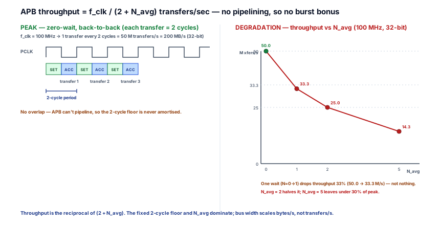
The throughput math of APB — transfers per second is f_clk/(2 + N_avg) with no burst bonus, so it is dominated by the fixed two-cycle floor and the average wait count, and it is deliberately modest because APB is a sparse control bus, not a bulk-data path.
Chapter 14.1 pinned the unit cost: one APB transfer is 2 + N cycles. This chapter turns that atom into a rate. Throughput is nothing more than the reciprocal of per-transfer latency: transfers/sec = f_clk / (2 + N_avg), and bytes/sec = bus_width_bytes × f_clk / (2 + N_avg). The single idea to carry: because APB cannot pipeline, there is no burst amortisation — back-to-back transfers each pay their own full 2 + N, so throughput is dominated by the fixed two-cycle floor and the average wait count, and nothing else. At 100 MHz the absolute ceiling is f_clk/2 = 50 M transfers/sec (200 MB/s on a 32-bit bus), and every wait state pushes it down a predictable amount. APB throughput is deliberately modest — it is a control bus, not a data mover — and once you can compute it, the whole utilisation and DMA-versus-CPU story becomes arithmetic.
1. Problem statement
The problem is computing how many transfers (and bytes) per second an APB link actually delivers — a hard number you can size a subsystem against, not a vague "it's slow."
A clock frequency alone tells you nothing useful. APB at 100 MHz is not 100 M transfers/sec; the two-phase structure and wait states cut it down, and the cut is exact:
- Throughput is the reciprocal of latency. From 14.1, one transfer costs
2 + Ncycles. A steady stream of transfers, each costing2 + N_avgcycles, completes one every2 + N_avgclocks — so the rate isf_clk / (2 + N_avg)transfers per second. That is the whole formula; everything else is plugging in numbers. - Bytes/sec adds one factor: the bus width. Each transfer moves
bus_width_bytes(4 on a 32-bit bus). Sobytes/sec = bus_width_bytes × f_clk / (2 + N_avg). Width scales the bytes per transfer, never the number of transfers per second. - The denominator is the whole story.
f_clkand width are usually fixed by the SoC; the lever is2 + N_avg. The fixed2is the floor you can never beat, andN_avgis the average wait count that pushes you below it. Throughput is therefore bounded above byf_clk/2and degrades monotonically asN_avggrows.
So the job is: given f_clk, bus width, and the average wait count N_avg, compute transfers/sec and bytes/sec — and know that the answer is f_clk / (2 + N_avg), with no pipelining bonus hiding anywhere.
2. Why previous knowledge is insufficient
You can already cost a single APB transfer at 2 + N cycles — that is exactly what Chapter 14.1, APB latency anatomy established, and what the multi-wait chapter taught you about driving PREADY low for several cycles. What you have not done is aggregate that single cost into a rate:
- Latency is a per-transfer number; throughput is the steady-state rate. Knowing one transfer costs
2 + Ncycles does not, by itself, tell you transfers/sec — you need to multiply byf_clkand divide by the per-transfer cost, and decide whatNto use across a stream (the average,N_avg). The shift is from "this transfer cost 3 cycles" to "this link sustainsf_clk/(2+N_avg)transfers per second." - The tempting (wrong) instinct is to amortise the floor across a burst. On a pipelined bus, back-to-back transfers overlap and the fixed cost gets hidden. APB cannot do this — and why it can't is the subject of Chapter 14.3, why APB is not pipelined. For this chapter you take that as given: each transfer pays its own full
2 + N, so the per-transfer cost in a stream is the same as in isolation, and there is no burst bonus to divide out. - Peak throughput is not the same as achieved utilisation. This chapter computes the peak and steady-state rate the protocol can deliver for a given
N_avg. What fraction of that a real workload actually uses — idle gaps, bursty arrival, contention — is Chapter 14.4, bus utilisation. Keep them separate: here we ask "how fast can it go for thisN_avg?", not "how busy is it?"
So the model to add is the aggregate: take the 2 + N atom, average the wait count over a stream, and turn it into f_clk / (2 + N_avg) — the rate the rest of the performance module multiplies and budgets against.
3. Mental model
The model: APB is a metronome with a fixed two-beat minimum. Every transfer takes at least two beats (SETUP + ACCESS), and a slow slave adds N extra wait beats. The metronome never lets two transfers share beats — no overlap, ever — so the rate at which transfers complete is simply one transfer per (2 + N_avg) beats, and the beats tick at f_clk. Count the beats per transfer, divide the clock by it, and you have the throughput.
Three refinements make it exact:
- Peak is
f_clk / 2. With zero waits (N_avg = 0), every transfer is two beats, so one completes every two clocks:f_clk/2transfers/sec. At 100 MHz that is 50 M transfers/sec — the absolute ceiling, hit only by an always-ready slave. There is no faster APB. - Waits push the denominator up, fast.
N_avg = 1makes itf_clk/3;N_avg = 2makes itf_clk/4— already half of peak. Because the floor is only2, a smallN_avgis a large relative cost: going fromN_avg = 0to1is a 33% throughput loss, not a rounding error. The reciprocal relationship makes early waits bite hard. - Width multiplies bytes, never transfers. A 32-bit bus moves 4 bytes/transfer, a 64-bit bus 8 — so
bytes/secdoubles, buttransfers/secis identical (f_clk/(2+N_avg)regardless of width). Width buys you bandwidth per transfer, not more transfers. This is why APB stays modest: even a wide, fast, zero-wait APB tops out at a control-bus-grade data rate.
4. Real SoC implementation
In practice you do two things with this formula. In RTL or a monitor you count completed transfers per time window to measure achieved throughput; in a budgeting spreadsheet (or firmware sizing code) you compute the rate from f_clk, width, and N_avg. Here is the worked calculation — the arithmetic an architect runs to size an APB link, written as a small, commented C snippet.
// Compute APB throughput from clock, bus width, and average wait count.
// Throughput is the reciprocal of per-transfer latency: f_clk / (2 + N_avg).
// There is NO burst bonus — APB cannot pipeline, so every transfer pays 2 + N.

double f_clk_hz   = 100e6;   // 100 MHz APB clock
double width_bits = 32;      // 32-bit data bus
double n_avg      = 0.0;     // average wait states per transfer (sweep this)

double width_bytes = width_bits / 8.0;          // 4 bytes per transfer (32-bit)

// transfers/sec = f_clk / (2 + N_avg)   -- the 2 is the fixed SETUP+ACCESS floor
double xfers_per_sec = f_clk_hz / (2.0 + n_avg);

// bytes/sec = bus_width_bytes * f_clk / (2 + N_avg)
double bytes_per_sec = width_bytes * xfers_per_sec;
double mb_per_sec    = bytes_per_sec / 1e6;     // decimal MB/s

// Worked results at 100 MHz, 32-bit (width_bytes = 4):
//   N_avg = 0  ->  100e6/2 = 50.0 M xfers/s  -> 200.0 MB/s   <- PEAK (f_clk/2)
//   N_avg = 1  ->  100e6/3 = 33.3 M xfers/s  -> 133.3 MB/s
//   N_avg = 2  ->  100e6/4 = 25.0 M xfers/s  -> 100.0 MB/s   <- already half of peak
//   N_avg = 5  ->  100e6/7 = 14.3 M xfers/s  ->  57.1 MB/s
//
// Same N_avg=0 on a 64-bit bus (width_bytes = 8):
//   transfers/sec is UNCHANGED at 50.0 M/s; only bytes/sec doubles to 400 MB/s.
Two facts make this the right way to size APB. First, N_avg is the only variable that moves the transfer rate — f_clk and width are SoC-fixed, so the whole sizing exercise is estimating the average wait count of the addressed slaves and reading off f_clk/(2+N_avg). Second, width and transfer rate are orthogonal: doubling the bus doubles bytes/sec but leaves transfers/sec exactly where it was, which is precisely why a wide APB is still a control bus — it cannot out-transfer the 2 + N_avg floor. To measure achieved throughput rather than compute peak, the RTL counterpart is a counter that increments on each (penable && pready) completion and is sampled every fixed window (xfers_this_window / window_seconds), feeding the utilisation math downstream.
5. Engineering tradeoffs
The formula is fixed (f_clk / (2 + N_avg)), so the tradeoffs are entirely about what N_avg and width do to the delivered rate. The table below sweeps N_avg at a fixed 100 MHz / 32-bit config, then shows the width effect — making the degradation and the orthogonality concrete.
| Config (100 MHz) | N_avg | Denominator 2 + N_avg | Transfers/sec | Bytes/sec (MB/s) | vs peak |
|---|---|---|---|---|---|
| 32-bit | 0 | 2 | 50.0 M | 200.0 | 100% (peak) |
| 32-bit | 1 | 3 | 33.3 M | 133.3 | 67% |
| 32-bit | 2 | 4 | 25.0 M | 100.0 | 50% |
| 32-bit | 5 | 7 | 14.3 M | 57.1 | 29% |
| 64-bit | 0 | 2 | 50.0 M (unchanged) | 400.0 (2×) | 100% transfers, 2× bytes |
| 64-bit | 2 | 4 | 25.0 M (unchanged) | 200.0 | 50% transfers, 2× bytes |
Two throughlines. First, the transfer rate column collapses fast with N_avg — one average wait already costs a third, two waits halve it, five leave under 30% of peak; because the floor is only 2, every wait is a large fraction of the denominator. Second, width moves only the bytes column — the 64-bit rows have identical transfers/sec to their 32-bit counterparts; widening the bus buys bandwidth per transfer, not a faster cadence. So if you need more transfers per second, you must reduce N_avg (or raise f_clk); if you need more bytes, you can also widen — but neither buys APB out of being a modest control bus, because the 2 + N_avg floor caps the transfer cadence regardless.
6. Common RTL mistakes
7. Debugging scenario
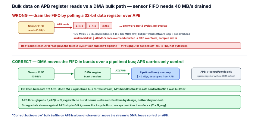
The signature throughput bug is a bus-choice error: someone routed a high-bandwidth data stream through APB register reads and got a fraction of the rate they needed — the anatomy of APB throughput is exactly what diagnoses it.
- Observed symptom: a driver draining a sensor sample FIFO (the stream produces 40 MB/s and must be emptied to avoid overflow) is losing samples — the FIFO periodically overflows and the
OVERFLOWstatus bit sets. Functionally each read returns correct data; the system simply cannot keep up, so data is dropped. - Waveform clue: tracing the APB shows the firmware polling a 32-bit data register one transfer at a time, each costing
2 + N = 3cycles (the FIFO read interface adds one wait,N = 1). The transfers are back-to-back but never overlap — there is no pipelining — so even fully saturated the link delivers only100 MHz / 3 = 33.3 Mreads/sec, and once the per-word software loop and poll overhead are counted the sustained drain falls well below the 40 MB/s the stream needs. The bus is busy yet under-delivering. - Root cause: bulk data was sized against a naive "bytes per clock" assumption that ignored the two-cycle floor and the lack of pipelining. APB throughput is
f_clk/(2 + N_avg)per transfer, with no burst amortisation — so per-word register reads can never match a streaming source. The error is architectural: a data mover's traffic was placed on a control bus. - Correct RTL: keep the bulk stream off APB. Add a DMA engine that moves the FIFO contents in bursts over a pipelined bus (AHB/AXI), decoupled from APB and easily exceeding 40 MB/s; leave APB to carry only the sparse control/configuration registers (including the DMA setup) it was designed for. Where the per-transfer wait is spurious (an over-conservative FIFO
PREADY), reducingNhelps marginally — but it cannot close a streaming gap, so the real fix is the bulk path, not shaving a wait. - Verification assertion: assert the achieved transfer rate meets the drain requirement, and cover that the FIFO never overflows under the chosen path. A throughput coverpoint plus a deadline assertion turns the overflow from a silent data loss into a caught regression:
// Throughput / drain check for the FIFO-on-APB scenario.
// Count completed APB reads in a window; assert the rate clears the drain need.
int unsigned xfers_in_window;
always_ff @(posedge pclk or negedge presetn)
  if (!presetn)                 xfers_in_window <= 0;
  else if (window_tick)         xfers_in_window <= 0;            // reset each window
  else if (penable && pready)   xfers_in_window <= xfers_in_window + 1;

// Required: >= MIN_XFERS reads per window to drain 40 MB/s without overflow.
ap_drain_rate: assert property (@(posedge pclk) disable iff(!presetn)
  window_tick |-> (xfers_in_window >= MIN_XFERS_PER_WINDOW));

// And the FIFO must never overflow under the chosen path.
ap_no_overflow: assert property (@(posedge pclk) disable iff(!presetn)
  !fifo_overflow);

// Coverage: did we exercise the saturated (back-to-back) read stream at all?
cp_saturated: cover property (@(posedge pclk)
(penable && pready) ##1 (psel && !penable) ##1 (penable && pready));- Debug habit: when an APB path is "correct but can't keep up," compute its peak
f_clk/(2 + N_avg)and compare it to the required rate before touching anything. If peak is already below the requirement, no RTL tuning will save it — it is a bus-choice problem, and the answer is DMA + a pipelined bus for the stream, with APB left to its control traffic. Size againsttransfers × (2 + N_avg), never against bytes/clock.
8. Verification perspective
Throughput is a measured steady-state rate, so verification's job is to instrument it correctly, cover the wait-count regimes that move it, and regress peak-versus-achieved so a throughput drop trips before silicon.
- Measure steady-state throughput, not a single transfer. Bind a counter that increments on each
(penable && pready)completion and sample it over a fixed window:transfers/sec = xfers_in_window / window_seconds. Cross-check against the formula — a saturated zero-wait stream should measuref_clk/2; if it doesn't, the monitor (or the stimulus saturation) is wrong, and every downstream number is suspect. - Cover the
N_avgrange, not just one regime. Functional coverage should bin the per-window average wait count across zero-wait, light-wait, and heavy-wait regimes, because throughput is a strong function ofN_avg. A suite that only ever runs the fast-register (N_avg ≈ 0) case reports the optimisticf_clk/2and never exercises the slow-slave throughput that real traffic sees — the performance hole hides behind functional green. - Assert peak-vs-achieved and regress it. For throughput-critical paths, assert the measured rate clears the required minimum (
xfers_in_window >= MIN_XFERS_PER_WINDOWfor the workload'sN_avg) and record the achieved rate as a regression metric. This catches a throughput regression — a new wait state, an over-conservativePREADY, a slave moved behind a CDC — that silently dropsf_clk/(2+N_avg)below budget. Peak is the ceiling; the assertion guards the floor of acceptable achieved rate.
The point: instrument throughput as a windowed measurement, cover the N_avg distribution that drives it, and assert achieved-versus-required so a throughput drop is regressed, not discovered in the lab.
9. Interview discussion
"What's the throughput of APB?" is a precision filter exactly like the latency question. The weak answer is "it's slow" or "around the clock rate"; the strong answer is the formula, the peak, and why there's no burst bonus.
State it exactly: APB throughput is f_clk / (2 + N_avg) transfers per second, and bus_width_bytes × f_clk / (2 + N_avg) bytes per second — the reciprocal of the 2 + N per-transfer latency from the cost model. Then deliver the depth: peak is f_clk/2 (zero waits, e.g. 50 M transfers/sec = 200 MB/s on a 32-bit bus at 100 MHz), because the two-phase floor is mandatory; waits degrade it sharply (N_avg = 1 is a 33% loss, N_avg = 2 halves it) because the denominator starts at only 2; there is no burst bonus — APB can't pipeline, so each transfer pays its own 2 + N and back-to-back streams don't amortise the floor; and width scales bytes/sec but not transfers/sec. The senior flourish ties it to design intent: "APB's throughput is low by design — it's a control bus for sparse register traffic, where simplicity and timing closure beat bandwidth; bulk data goes on DMA + a pipelined bus, and the moment someone needs streaming throughput on APB it's a bus-choice error, not a tuning problem." Saying "throughput is just f_clk/(2+N_avg), dominated by the floor and the average wait, with no pipelining to hide behind" signals you have actually sized an APB subsystem.
10. Practice
- Compute the peak. At an 80 MHz APB clock with a 32-bit bus and zero waits, give peak transfers/sec and MB/s. State the formula you used.
- Apply a wait. For the same 80 MHz / 32-bit link with
N_avg = 2, compute transfers/sec and MB/s, and the percentage of peak. - Isolate the width effect. Take the
N_avg = 1, 100 MHz case and give transfers/sec and bytes/sec for a 32-bit and a 64-bit bus. State which number changes and which doesn't, and why. - Disprove the burst bonus. A burst of 10 back-to-back zero-wait transfers: give the total cycles and the effective per-transfer cost, and explain why it's not less than
2per transfer. - Size a stream. A peripheral must sustain 120 MB/s on a 100 MHz, 32-bit APB. Compute the required transfers/sec, the
N_avgthat would deliver it, and state whether APB can meet it — and what you'd do if it can't.
11. Q&A
12. Key takeaways
- APB throughput is
f_clk / (2 + N_avg)transfers per second, andbus_width_bytes × f_clk / (2 + N_avg)bytes per second — the plain reciprocal of the2 + Nper-transfer latency, with no other terms. - Peak is
f_clk/2(zero waits): 50 M transfers/sec = 200 MB/s on a 32-bit bus at 100 MHz. The two-cycle floor is mandatory, so there is no faster APB and "100 MHz ≠ 100 M transfers/sec." - Waits degrade it sharply. Because the denominator starts at
2,N_avg = 1is a 33% loss andN_avg = 2halves throughput. The fixed floor andN_avgdominate everything. - No burst bonus. APB cannot pipeline, so back-to-back transfers each pay their own
2 + N; throughput is never amortised across a stream. Bursty/streaming traffic belongs on a pipelined bus. - Width scales bytes, not transfers. Doubling the bus doubles
bytes/secbut leavestransfers/sec = f_clk/(2+N_avg)unchanged — bandwidth per transfer, not a faster cadence. - APB is modest by design — and that's correct. It is a control bus for sparse register traffic; size data streams as
transfers × (2 + N_avg)and move bulk to DMA, then verify achieved throughput against the requirement so a regression is caught, not discovered.