Pipelining Benefit

Chapter 14.1 noted the address-phase overhead; this chapter quantifies how the AHB pipeline hides it. The mechanism: the next transfer's address phase overlaps the current transfer's data phase, so once the pipeline is full, the bus delivers one data beat per cycle — the address-phase overhead is hidden under the previous data phase. The quantified gain: a stream of N transfers takes ~N+1 cycles pipelined (1 to fill + N data beats) versus 2N cycles non-pipelined (address + data, sequentially) — approaching 2× throughput for long streams. But the benefit holds only when the pipeline stays full: an idle cycle (no transfer issued) leaves a bubble, a wait state stalls both phases, and an isolated single transfer gets no overlap (~50% efficient, chapter 14.1). So realizing the benefit means keeping transfers back-to-back (ideally bursts). Note: the benefit is throughput, not latency — each transfer still takes its 2 phases (chapter 14.2); pipelining overlaps successive transfers, raising the rate, not shortening any one. This chapter quantifies the gain and its conditions.

1. What Is It?

The pipelining benefit is the throughput gain from overlapping successive transfers' phases. Quantified:

• The overlap: the next transfer's address phase happens during the current transfer's data phase — so they don't serialize.
• Full-pipeline rate: once filled, one data beat per cycle (the address-phase overhead is hidden).
• The gain: N transfers ≈ N+1 cycles pipelined (1 fill + N data) vs 2N non-pipelined → up to 2× for long streams.
• The condition: the pipeline must stay full (back-to-back transfers); bubbles (idle), wait states, and isolated transfers lose the gain.

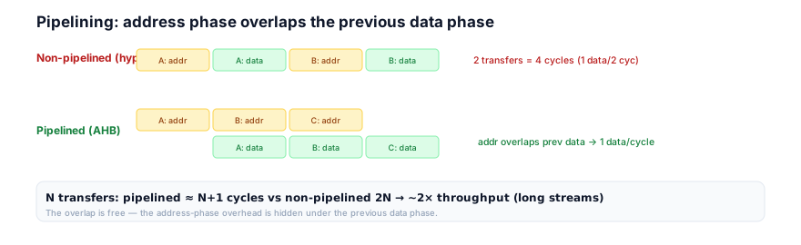
So the pipelining benefit is the hiding of the address-phase overhead: instead of paying an address cycle and a data cycle per transfer (non-pipelined, 2 cycles each), the pipeline overlaps the next address phase with the current data phase, so steady-state you pay one cycle per transfer (the address phase is "free," hidden under the previous data phase). This nearly doubles throughput for a continuous stream. It's the AHB pipeline (chapter 5.x) viewed through a performance lens — the address/data overlap isn't just how the protocol works, it's a 2× throughput optimization built into the protocol. So the pipelining benefit is the quantified throughput gain (up to 2×) from the address/data overlap, realized when the pipeline stays full.

2. Why Does It Exist?

The pipelining benefit exists because the address-phase overhead is fixed per transfer but independent of the data phase — so overlapping the next address phase with the current data phase hides the overhead, and this overlap is built into the AHB protocol precisely to get this throughput gain.

The fixed-but-overlappable overhead is the root: every transfer needs an address phase (to tell the slave what to do) — a fixed 1-cycle cost. Without overlap, this cost is added to each transfer (address cycle + data cycle = 2 cycles/transfer), halving throughput. But the address phase of the next transfer is independent of the data phase of the current one — the master can drive the next address while the current data is being transferred (different signals, no conflict). So the overhead can be overlapped with useful data work. So the benefit exists because the overhead is hideable — it doesn't have to be serial. So overlapping it is possible.

The built-into-the-protocol point: AHB's two-phase pipeline (chapter 5.x) is designed so the address phase and data phase are separate, overlappable phases — precisely so successive transfers can overlap. The protocol defines that while a transfer is in its data phase, the next is in its address phase. So the overlap isn't an add-on; it's the structure of AHB. And the reason it's structured this way is throughput — the protocol designers built in the pipeline to get the ~2× gain over a non-pipelined bus. So the pipelining benefit exists because AHB's pipeline is this overlap, designed for throughput. So it's intrinsic to the protocol.

The reason it's conditional (only when full) is that the overlap requires a continuous stream: the next address phase can only overlap the current data phase if there is a next transfer ready to issue. If the master doesn't issue (idle), there's a bubble (no overlap that cycle). If the slave stalls (wait state), both phases hold (no progress). If there's only one transfer (isolated), there's no next to overlap (it's just address + data = 2 cycles, 50% efficient). So the benefit is realized only when the pipeline is kept full — back-to-back transfers. So the conditionality exists because the overlap needs a continuous supply of transfers. So the pipelining benefit exists because: the address-phase overhead is fixed-per-transfer but overlappable with the data phase (the opportunity), the AHB protocol is designed around this overlap for throughput (the mechanism), and it's realized only when the pipeline stays full (the condition — back-to-back transfers/bursts). It's the protocol's built-in ~2× throughput optimization, contingent on keeping transfers flowing. So this chapter quantifies how much (N+1 vs 2N → 2×) and when (full pipeline) — guiding the design toward back-to-back, bursted traffic.

3. Mental Model

Model the pipelining benefit as a car wash with a wash bay and a drying bay — without pipelining, each car is washed then dried then leaves before the next enters (two stations' time per car); with pipelining, as soon as a car moves from washing to drying, the next car enters the wash bay — so once the line is going, a finished car comes out every "drying time," nearly doubling the cars-per-hour; but the benefit only holds if cars keep arriving back-to-back — a gap in the line (idle), a car stuck in a bay (wait state), or just one lone car (no follow-on) loses the overlap.

A car wash has two stations: a wash bay (the address phase — the setup) and a drying bay (the data phase — the result). Without pipelining, one car is washed, then dried, then leaves, and only then does the next car enter — so each car ties up the whole line for two stations' worth of time; the cars-per-hour is low. With pipelining, as soon as a car moves from the wash bay to the drying bay, the next car immediately enters the wash bay — so the two bays are both busy (one washing the next car, one drying the current). Once the line is going, a finished car exits every drying-time — the wash time is hidden (happening in parallel with the previous car's drying). This nearly doubles the cars-per-hour. But — and this is the catch — the benefit only holds if cars keep arriving back-to-back: a gap in the line (no car arrives — an idle cycle) leaves a bay empty (a bubble, lost throughput); a car stuck in a bay (a breakdown — a wait state) stalls the whole line; and just one lone car (no follow-on) gets no overlap — it's washed and dried with no parallelism (the 50% case). So the throughput nearly doubles only with a continuous stream of cars.

This captures the pipelining benefit: the wash bay and drying bay = the address and data phases; washing then drying sequentially = non-pipelined (2 cycles/transfer); next car entering as the current moves to drying = the address phase overlapping the previous data phase; a finished car every drying-time = one data beat per cycle (full pipeline); nearly doubling cars-per-hour = ~2× throughput; a gap in the line = an idle bubble; a stuck car = a wait state; one lone car = an isolated transfer (50%). Two bays both busy on a continuous stream — that's the pipelining benefit.

Watch the pipeline deliver one beat per cycle when full:

The model's lesson: two bays both busy on a continuous stream — a finished car every drying-time. In the waveform, each address phase overlaps the previous data phase, so data comes out every cycle once the pipeline fills — the ~2× throughput gain.

4. Real Hardware Perspective

In hardware, the pipelining benefit comes free from the AHB protocol's phase structure — the master just issues transfers back-to-back and the overlap happens automatically — but realizing it requires the master to sustain the issue rate and the slaves to be zero-wait.

The automatic overlap: the AHB protocol's phase structure (chapter 5.x) inherently overlaps the next address phase with the current data phase — the master drives the next HADDR/HTRANS while the current transfer's data is on HRDATA/HWDATA. So the hardware gets the overlap for free — no special logic; it's how the bus works. So the pipelining benefit is built in. So a master issuing back-to-back transfers automatically pipelines them.

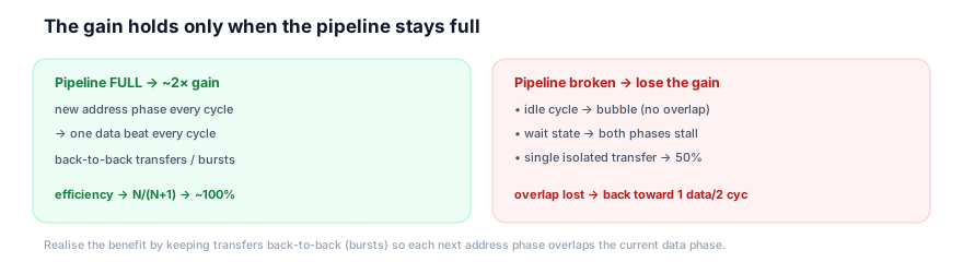
The sustaining the issue rate is the master's job: to keep the pipeline full, the master must issue a new transfer every cycle (a new address phase each cycle). This requires the master to have transfers ready — e.g. a burst (HBURST, chapter 8.x) where the addresses are known (incrementing/wrapping), so the master issues them back-to-back without computing each. Or a master with a deep request queue / prefetch. If the master can't sustain (must compute the next address, wait for data, re-arbitrate), it inserts bubbles (idle cycles), losing the benefit. So in hardware, bursts are the natural way to sustain the issue rate — the master streams a known address sequence. So bursts realize the pipelining benefit.

The zero-wait slaves are the other condition: a wait state (slave not ready) stalls the pipeline — both the current data phase and the next address phase hold (no progress that cycle). So wait states break the one-beat-per-cycle rate. So to sustain the benefit, the slaves must be fast (zero-wait) — a slow slave (wait states) reduces the effective rate below 1 beat/cycle (chapter 14.4 quantifies the wait-state penalty). So in hardware, the pipelining benefit is automatic from the protocol but realized only when the master sustains back-to-back issue (bursts, queues) and the slaves are zero-wait. The overlap is free; keeping it going is the design effort. So in hardware, pipelining gives ~2× throughput for streams that keep the pipeline full — and bursts to fast slaves are the canonical way to achieve that. So the hardware benefit is the protocol's free overlap, realized by sustained back-to-back, zero-wait traffic.

5. System Architecture Perspective

At the system level, the pipelining benefit is why bursts to fast memory are the canonical high-bandwidth pattern — it's the protocol-level half of the throughput story (the other half being width/clock and concurrency), and it shapes how bandwidth-bound traffic is structured.

The canonical high-bandwidth pattern: the pipelining benefit means that the way to get near-peak throughput on AHB is to issue back-to-back transfers to zero-wait slaves — which in practice means bursts to fast memory. A burst (chapter 8.x) gives the master a known address sequence to issue back-to-back (keeping the pipeline full), and a fast memory (SRAM, or cached) provides zero-wait data (sustaining one beat/cycle). So burst-to-fast-memory is the high-throughput idiom, and it works because of the pipelining benefit (the overlap hides the address overhead). So at the system level, the pipelining benefit motivates structuring bandwidth-bound traffic as bursts to fast memory. So it shapes the data-movement design.

The protocol-level throughput half: the pipelining benefit is the protocol-level contribution to throughput — it's what gets a single AHB path from ~50% (isolated transfers) toward ~100% efficiency (full pipeline). The other throughput levers are physical (bus width, clock — the peak, chapter 14.1) and architectural (concurrency — the matrix, Module 13). So the full throughput story is: physical peak (width × clock) × protocol efficiency (pipelining → ~100% if full) × architectural concurrency (matrix → aggregate across slaves). So the pipelining benefit is the efficiency multiplier on a single path. So at the system level, it's one of three composable throughput factors (peak, pipeline-efficiency, concurrency). Understanding it lets the architect separate the throughput contributions — and recognize that pipelining gets a single path near 100% efficiency, but aggregate bandwidth beyond one path's peak needs a matrix.

The interaction with the other effects: the pipelining benefit composes with (and is limited by) the later chapters' effects. Wait states (chapter 14.4) break the pipeline (reduce below 1 beat/cycle) — so the pipelining benefit assumes zero-wait. Bursts (chapter 14.5) are how you sustain the full pipeline (and amortise the fill cost). Arbitration (chapter 14.6) can insert bubbles (re-arbitration gaps) breaking the pipeline. Bridges (chapter 14.7) add latency and may break the pipeline (APB is non-pipelined). So the pipelining benefit is the baseline throughput model, and the other effects are deviations from it (each reducing the realized benefit). So at the system level, the pipelining benefit is the canonical high-bandwidth pattern's foundation (bursts to fast memory), the protocol-level efficiency factor in the composable throughput story (peak × pipeline-efficiency × concurrency), and the baseline against which the other performance effects (waits, bursts, arbitration, bridges) are measured as deviations. So it's the central throughput mechanism on a single path — get the pipeline full (bursts, fast slaves, no bubbles) and you get ~2× over non-pipelined, approaching the path's peak. So the pipelining benefit anchors the throughput analysis of the whole module.

6. Engineering Tradeoffs

The pipelining benefit embodies the overlap-the-overhead, keep-the-pipeline-full design.

• Pipelined stream vs isolated transfers. A back-to-back stream (full pipeline) gets ~2× throughput (1 beat/cycle); isolated single transfers get ~50% (2 cycles each). Stream transfers (bursts) for bandwidth.
• Bursts (sustain the pipeline) vs single transfers. Bursts give a known address sequence to issue back-to-back, keeping the pipeline full and amortising the fill cost; single transfers can't sustain it. Use bursts for the pipelining benefit.
• Fast slaves (no stall) vs slow slaves. Zero-wait slaves sustain one beat/cycle; slow slaves (wait states) break the pipeline (chapter 14.4). Fast slaves are needed to realize the benefit.
• Throughput gain, not latency. Pipelining raises throughput (the rate) but doesn't reduce per-transfer latency (each still takes its 2 phases, chapter 14.2). It helps streaming, not single dependent accesses.

The throughline: the AHB pipeline overlaps the next transfer's address phase with the current transfer's data phase, so once full, the bus delivers one data beat per cycle — hiding the address-phase overhead. N transfers take ~N+1 cycles (pipelined) vs 2N (non-pipelined) → up to ~2× throughput for long streams. The benefit holds only when the pipeline stays full (back-to-back transfers / bursts to zero-wait slaves); idle cycles, wait states, and isolated transfers break the overlap. It's a throughput gain (not latency), it's automatic from the protocol but realized by sustained back-to-back issue, and it's the foundation of the canonical burst-to-fast-memory high-bandwidth pattern.

7. Industry Example

Quantify the pipelining benefit for a DMA stream.

A DMA copies a buffer on a 32-bit AHB bus; compare pipelined vs non-pipelined.

• Non-pipelined (hypothetical baseline). If each transfer were address-then-data sequentially, copying N words would take 2N cycles (N address + N data, serialized). At 100 MHz, copying 1000 words = 2000 cycles = 20 µs. Throughput ≈ 200 MB/s (50% of the 400 MB/s peak).
• Pipelined, full (bursts to fast SRAM). The DMA issues an incrementing burst (back-to-back, addresses known) to a zero-wait SRAM. The pipeline fills after 1 cycle, then delivers 1 word/cycle. Copying 1000 words ≈ 1001 cycles ≈ 10 µs. Throughput ≈ 400 MB/s (≈100% of peak). The pipelining benefit ≈ 2× over non-pipelined.
• Pipeline broken by bubbles (counter-example). If the DMA stalled between transfers (e.g. fetching descriptors, re-arbitrating, computing each address with single transfers), it would insert bubbles — say one idle cycle per transfer — dropping back toward 1 beat per 2 cycles (~200 MB/s). The benefit is lost because the pipeline isn't full.
• Pipeline broken by wait states. If the target were slow flash (say 1 wait state per beat), each beat takes 2 cycles, halving the rate (~200 MB/s) — the pipeline can't sustain 1 beat/cycle. So a fast (zero-wait) slave is needed.
• Realizing the benefit. The DMA is designed to issue long bursts back-to-back (deep queues, known burst addresses) to fast SRAM — keeping the pipeline full, achieving ~100% efficiency and the full ~2× pipelining benefit.
• Latency unchanged. Note: each individual word's latency (address + data) is unchanged by pipelining — the DMA's throughput doubled, but a single word's transfer time didn't. (The DMA cares about throughput, so this is fine.)

The example quantifies the benefit: ~2× throughput (200 → 400 MB/s) from keeping the pipeline full (bursts to fast SRAM), lost if bubbles or wait states break the overlap. The pipelining benefit is realized by sustained back-to-back, zero-wait streaming — the canonical high-bandwidth pattern. This is how the pipeline's throughput gain is computed and achieved.

8. Common Mistakes

9. Interview Insight

The pipelining benefit is a quantitative interview topic — the overlap mechanism, the N+1-vs-2N math, and the full-pipeline condition are the signals.

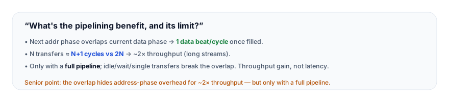
The answer that lands gives the mechanism, the math, and the condition: "The AHB pipeline overlaps the next transfer's address phase with the current transfer's data phase. So once the pipeline is full, after the first address phase, the bus delivers one data beat every cycle — the address-phase overhead is hidden under the previous transfer's data phase. Quantitatively: a stream of N transfers takes about N+1 cycles pipelined — one cycle to fill plus N data beats — versus 2N cycles if you did each transfer's address then data sequentially. So for long streams, that's nearly a 2× throughput gain. The crucial condition is that the pipeline must stay full: you need a new transfer issued every cycle. If the master goes idle, you get a bubble; if the slave inserts a wait state, both phases stall; and an isolated single transfer has no follow-on to overlap, so it's just 2 cycles, 50% efficient. So you realize the benefit by keeping transfers back-to-back — typically with bursts, where the address sequence is known so the master can issue continuously — to zero-wait slaves. And importantly, this is a throughput gain, not a latency reduction: each transfer still takes its two phases; pipelining raises the rate of a stream, it doesn't speed up any single transfer. So it helps streaming workloads like DMA, not single dependent accesses." The overlap mechanism, the N+1-vs-2N math, the full-pipeline condition, and the throughput-not-latency point are the senior signals.

10. Practice Challenge

Compute and reason from the pipelining benefit.

1. The math. Compute the cycles for a 16-transfer stream pipelined (full) vs non-pipelined, and the speedup.
2. The mechanism. Explain how the address/data overlap delivers one beat per cycle.
3. Read the waveform. From Figure 2, identify where each address phase overlaps the previous data phase.
4. What breaks it. Name three things that break the full pipeline and lose the benefit.
5. Throughput not latency. Explain why pipelining helps a DMA stream but not a single dependent CPU load.

11. Key Takeaways

• The pipeline overlaps the next transfer's address phase with the current transfer's data phase — so once full, the bus delivers one data beat per cycle (the address-phase overhead is hidden).
• The gain: N transfers ≈ N+1 cycles (pipelined) vs 2N (non-pipelined) → up to ~2× throughput for long streams (efficiency N/(N+1) → ~100%).
• It's a throughput gain, NOT a latency reduction — each transfer still takes its 2 phases; pipelining raises the rate of a stream, not the speed of any one transfer.
• It holds only when the pipeline stays full — idle cycles (bubbles), wait states, and isolated single transfers break the overlap and lose the gain (a lone transfer is ~50% efficient).
• Realize it with back-to-back transfers — typically bursts (known address sequence) to zero-wait slaves — the canonical burst-to-fast-memory high-bandwidth pattern.
• It's the protocol-level efficiency factor in the composable throughput story (peak × pipeline-efficiency × concurrency) — getting a single path from ~50% toward ~100% efficiency.

12. What Comes Next

You now understand the pipelining benefit — the ~2× throughput gain from the phase overlap, realized when the pipeline stays full. The next chapters quantify the deviations from this ideal:

• Wait-State Penalty (next) — quantifying how wait states erode throughput (break the pipeline).
• Burst Efficiency — how bursts amortise the address-phase overhead (sustain the pipeline).
• Arbitration Overhead, Bridge Penalty, Bottleneck Analysis, Performance Debug — the other effects and how to debug performance.

To revisit the pipeline structure this exploits, see Address & Data Phase; for the throughput context, see Throughput.