Wait-State Penalty

Chapter 14.3 showed the pipeline delivering one beat per cycle when full — and noted that wait states break it. This chapter quantifies that wait-state penalty. The mechanism: each wait state (HREADY low) is a no-data cycle — the slave isn't ready, so that cycle moves no payload. So a beat that takes W wait states occupies 1 + W cycles (1 data cycle + W waits), and the per-beat efficiency = 1/(1+W). The numbers are stark: W=1 halves throughput (50%), W=2 cuts it to a third (33%), W=4 to a fifth (20%). So wait states multiply the time-per-beat directly — which is why a slow slave is often the dominant throughput loss (more than address overhead or arbitration). And they break the pipeline (chapter 14.3): a wait state stalls both the current data phase and the next address phase, dropping below one beat/cycle. The remedies attack the wait states: caching/prefetch (serve the common case fast), faster memory (fewer/no waits), or a wider bus (more data per surviving cycle). This chapter quantifies the penalty and the mitigations.

1. What Is It?

The wait-state penalty is the throughput loss from a slave inserting wait states. Quantified:

• Each wait state = a no-data cycle (HREADY low — the slave isn't ready, no payload moves).
• Cycles per beat = 1 + W (1 data cycle + W wait states).
• Per-beat efficiency = 1/(1+W) — W=1 → 50%, W=2 → 33%, W=4 → 20%.
• It breaks the pipeline — a wait state stalls both phases, dropping below one beat/cycle.

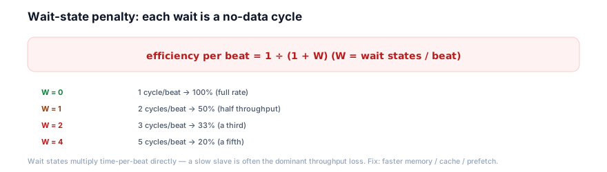
So the wait-state penalty is a direct multiplier on the time per beat: each wait state adds a full cycle that carries no data, so W wait states turn a 1-cycle beat into a (1+W)-cycle beat. The efficiency 1/(1+W) falls quickly — even one wait state halves throughput, and a few wait states devastate it. This is more severe than the address-phase overhead (which a burst amortises over many beats, chapter 14.1/14.5) — wait states are per beat and can't be amortised (every beat to a slow slave pays them). So a slow slave (many wait states per beat) is frequently the single biggest throughput loss in a system. So the wait-state penalty is the per-beat throughput multiplier (1/(1+W)) from a slave's wait states — often the dominant performance limiter.

2. Why Does It Exist?

The wait-state penalty exists because a wait state is a full cycle of no data — inherent to a slave needing more time — and because, unlike the address-phase overhead, wait states are per-beat and unamortisable, a slow slave's wait states multiply directly into throughput loss.

The wait state is a no-data cycle is the root: a wait state (HREADY low, chapter 12.4) means the slave isn't ready to complete the transfer this cycle — so no data moves. The cycle is spent waiting. So each wait state is, by definition, a cycle that carries no payload — a direct throughput loss (a cycle that could have carried a beat but didn't). So the penalty exists because wait states are lost data cycles. So W wait states = W lost cycles per beat.

The per-beat, unamortisable nature is why it's severe: the address-phase overhead is per-transaction (one address phase per burst) — so a burst amortises it over many beats (chapter 14.1/14.5), making it small for long bursts. But wait states are per beat — every beat to a slow slave pays its wait states, regardless of burst length. A 16-beat burst to a slave with 2 wait states/beat pays 2×16 = 32 wait cycles (plus 16 data + 1 address) — the wait states dominate, and the burst doesn't help (it amortises the address overhead, not the wait states). So wait states can't be amortised — they scale with the number of beats. So a slow slave's penalty is unavoidable per beat. So the penalty exists, severe and unamortisable, because it's per-beat. So this is why a slow slave is often the dominant loss.

The reason the efficiency is 1/(1+W) (the precise form) is the ratio of data to total cycles: a beat takes 1 data cycle + W wait cycles = 1+W total cycles, of which 1 carries data. So efficiency = data cycles / total cycles = 1/(1+W). So the formula is the data-fraction of the beat's cycles. And it falls fast because it's a reciprocal — adding wait states divides the throughput (W=1 → ÷2, W=2 → ÷3). So the penalty exists with this reciprocal severity because each wait state adds to the denominator. So the wait-state penalty exists because: a wait state is inherently a no-data cycle (the slave needs time — the why), wait states are per-beat and unamortisable (unlike address overhead — so they scale with beats, the severity), and the efficiency 1/(1+W) is the data-fraction of the beat's cycles, falling reciprocally (the math). So a slow slave directly divides throughput, making it frequently the dominant loss — and the only fixes are to reduce the wait states themselves (faster slave, cache) or move more data per surviving cycle (wider bus). So this chapter quantifies why slow slaves hurt so much and how to fix them.

3. Mental Model

Model the wait-state penalty as a checkout line where the cashier sometimes pauses to look something up — every pause is dead time in which no items are scanned, so a customer who triggers 2 lookups per item takes 3× as long as one with none; and crucially, batching more items per customer (a burst) doesn't help, because each item still triggers its own lookups — the only fixes are a faster cashier (fewer lookups) or scanning more items at once (a wider belt).

A checkout line (the bus) scans items (data beats). Normally, the cashier scans one item per second (one beat per cycle). But sometimes the cashier pauses to look something up — a price check, an ID verification (a wait state) — and during each pause, no items are scanned (no data moves). So an item that triggers W lookups takes 1 + W seconds (1 to scan + W paused). If every item triggers 2 lookups, each takes 3 seconds — the line moves at one-third speed (efficiency 1/(1+2) = 33%). Crucially, batching more items per customer (a longer burst) does not help here: the paperwork to start a customer (the address phase) is amortised, yes, but each item still triggers its own lookups — so a 20-item customer with 2 lookups/item still pays 40 lookup-seconds. The lookups scale with items, unamortisable. The only real fixes: a faster cashier who doesn't need lookups (a faster slave — fewer wait states), or a wider belt that scans multiple items at once (a wider bus — more data per scanning second, partly offsetting the lookups). So the lookups are dead time that multiplies the per-item time, and you fix them by eliminating the lookups or scanning more per second.

This captures the wait-state penalty: scanning an item = a data beat (1 cycle); the cashier pausing to look up = a wait state (no-data cycle); W lookups per item → 1+W seconds = W wait states → 1+W cycles/beat; one-third speed = efficiency 1/(1+W); batching items not helping = bursts don't amortise wait states (per-beat); a faster cashier = a faster slave (fewer waits); a wider belt = a wider bus. Lookups are dead time multiplying per-item time — fix by faster cashier or wider belt.

Watch wait states halve the effective rate:

The model's lesson: lookups are dead time multiplying per-item time — fix by faster cashier or wider belt. In the waveform, the 1 wait state per beat halves the rate (data on every other cycle) — efficiency 1/(1+1) = 50%.

4. Real Hardware Perspective

In hardware, the wait-state penalty comes from slow slaves (flash, external memory, slow peripherals), and the mitigations are concrete memory-system techniques: caching, prefetch, faster memory, and wider buses.

The slow-slave sources: wait states come from slaves that can't complete in one cycle. Flash is the classic example — flash read latency (especially at high CPU clocks) requires multiple wait states (e.g. 3-5 at 100+ MHz). External memory (DRAM, off-chip) has long latencies (many wait states). Slow peripherals may insert waits. So in hardware, the wait-state penalty is a property of the slaves in the system — the slower the slave (relative to the bus clock), the more wait states, the bigger the penalty. So identify the slow slaves.

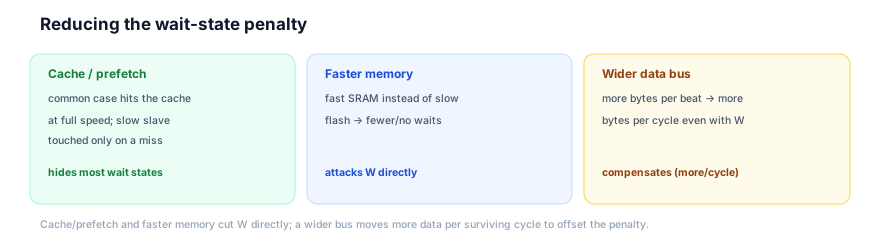
The caching/prefetch mitigation is the most powerful: a cache (or prefetch buffer) serves the common-case access at full speed (a cache hit is zero-wait), so the slow slave (flash, external memory) is touched only on a miss. For code/data with locality, the hit rate is high, so most accesses avoid the wait states. Flash accelerators (prefetch + small cache) are standard for exactly this — they hide flash's wait states for sequential code fetch. So in hardware, caching/prefetch is the primary wait-state mitigation. So add a cache for a slow, frequently-accessed slave.

The faster memory and wider bus: faster memory (fast SRAM instead of slow flash, or a faster memory grade) directly reduces W — fewer wait states per beat. A wider data bus (64-bit instead of 32-bit) compensates: even with wait states, each beat now moves twice the data, so the bytes/cycle (and thus throughput) rises — partly offsetting the penalty (you pay the same wait states but move more data per beat). So in hardware, the mitigations are: cache/prefetch (hide the waits for the common case), faster memory (cut W), and wider bus (more data per surviving beat). The choice depends on the slave (cache a frequently-accessed slow slave; widen the bus for a bandwidth-bound slow slave; use faster memory if affordable). So in hardware, the wait-state penalty is a slow-slave property, mitigated by the memory-system techniques (caching/prefetch, faster memory, wider bus) — and addressing it is often the highest-impact performance fix, since a slow slave can be the dominant loss. So the hardware reality: find the slow slave, hide or reduce its wait states.

5. System Architecture Perspective

At the system level, the wait-state penalty is usually the first thing to check in a throughput problem — because slow slaves (especially flash and external memory) are common and their penalty is severe — and the memory hierarchy exists largely to mitigate it.

The first thing to check: because the wait-state penalty is severe (reciprocal: even W=1 halves throughput) and unamortisable (per beat), a slow slave is frequently the dominant throughput loss — more than address overhead, arbitration, or anything else. So when a system is throughput-bound, the first analysis is usually "which slave is being accessed, and how many wait states does it insert?" — because a slow slave often is the bottleneck (chapter 14.8). So at the system level, the wait-state penalty is the prime suspect in a throughput problem. So check the slaves' wait states first.

The memory hierarchy as mitigation: the entire memory hierarchy — caches, prefetch buffers, fast on-chip SRAM, flash accelerators — exists largely to mitigate the wait-state penalty of slow backing stores (flash, external DRAM). A cache turns most accesses into zero-wait hits (hiding the slow store's waits); prefetch anticipates sequential access (hiding latency); fast SRAM for hot data avoids the slow store entirely. So the memory hierarchy is, in performance terms, a wait-state-hiding structure. So at the system level, mitigating the wait-state penalty is memory-hierarchy design — placing fast memory/caches between the masters and the slow stores. So the hierarchy exists to fight wait states.

The placement and budgeting: since wait states are so impactful, the architect budgets them — placing frequently-accessed, latency/throughput-critical data in fast (low-wait) memory, and tolerating wait states only for infrequent or latency-tolerant accesses. Hot code/data → cache or fast SRAM (low W); cold or bulk → can tolerate the slow store (high W) if accessed rarely. So the architect matches data placement to wait-state tolerance — a key performance-design decision. So at the system level, the wait-state penalty is the prime suspect in throughput problems (check the slaves first — slow slaves are often the dominant loss), the memory hierarchy (caches, prefetch, fast SRAM) exists largely to mitigate it, and data placement is budgeted against wait-state cost (hot data in fast memory, slow stores for cold/infrequent data). So the wait-state penalty drives much of memory-system architecture — it's the performance reason caches and fast memories exist, and the first thing to attack when throughput is short. So understanding 1/(1+W) and its unamortisable, reciprocal severity is central to performance engineering.

6. Engineering Tradeoffs

The wait-state penalty embodies the per-beat, unamortisable, reciprocal-severity loss.

• Reduce W (faster slave/cache) vs tolerate. Reducing wait states (faster memory, cache, prefetch) directly raises throughput (efficiency 1/(1+W) rises fast as W falls), at the cost of the faster memory / cache area. Worth it for frequently-accessed slow slaves (often the dominant loss).
• Cache/prefetch vs direct slow access. A cache hides most wait states (high hit rate → mostly zero-wait) at the cost of cache area/complexity; direct slow access pays the full penalty every time. Cache hot, slow-backed data.
• Wider bus vs same width. A wider bus moves more data per (wait-stated) beat, compensating for the penalty, at area cost; the same width pays the penalty on less data. Widen for bandwidth-bound slow slaves.
• Hot data in fast memory vs uniform placement. Placing hot/critical data in low-wait memory (and tolerating waits only for cold data) maximizes effective throughput; uniform placement (everything in the slow store) pays the penalty broadly. Budget placement by wait-state tolerance.

The throughline: each wait state is a no-data cycle, so a beat with W wait states takes 1+W cycles and per-beat efficiency = 1/(1+W) — W=1 halves throughput, W=2 cuts it to a third. Wait states multiply time-per-beat directly, are per-beat and unamortisable (bursts don't help — every beat pays), and break the pipeline — so a slow slave is often the dominant throughput loss. Mitigate by reducing W (faster memory, caching/prefetch — the memory hierarchy exists for this) or moving more data per surviving cycle (wider bus), and by placing hot data in fast memory. It's usually the first thing to check in a throughput problem.

7. Industry Example

Diagnose and fix a wait-state bottleneck.

A CPU fetches code from flash on a 32-bit AHB bus at 100 MHz; throughput is poor.

• Measure. The CPU's instruction-fetch throughput is ~100 MB/s — far below the 400 MB/s peak. Why?
• Find the wait states. The flash, at 100 MHz, inserts 3 wait states per access (flash is slow relative to the clock). So each fetch beat takes 1 + 3 = 4 cycles → efficiency 1/(1+3) = 25% → 0.25 × 400 = 100 MB/s. The wait-state penalty (W=3) is the dominant loss.
• Bursts don't help (the trap). One might try bursting the fetches. But the flash's 3 wait states are per beat — a burst amortises only the address overhead (negligible), not the wait states. So bursting keeps efficiency at ~25%. The burst is the wrong fix.
• Fix: flash accelerator (cache/prefetch). Add a flash accelerator — a small cache + prefetch buffer. Now sequential code fetches hit the prefetch/cache at full speed (zero-wait), and the slow flash is accessed only on the (rare) miss. The effective wait states drop toward 0 → efficiency toward 100% → throughput toward 400 MB/s. The accelerator hid the wait states.
• Alternative: run code from fast SRAM. Copy hot code to fast SRAM (zero-wait) and run from there — directly eliminating the flash wait states for that code. (Common for performance-critical routines.)
• Alternative: wider bus. A 64-bit bus would fetch 8 bytes per (3-wait-state) beat instead of 4 — doubling the bytes/cycle, so ~200 MB/s even with the waits. Helps, but caching is more effective (it removes the waits entirely for hits).
• Result. The flash accelerator (cache/prefetch) raises the effective throughput toward the peak by hiding the flash's wait states — the right fix for the wait-state bottleneck. Bursts alone would not have helped.

The example shows the wait-state penalty as the dominant loss (W=3 → 25% efficiency), the trap of trying bursts (which don't amortise wait states), and the right fix (cache/prefetch to hide the waits, or fast SRAM to avoid them). This is how a wait-state bottleneck is diagnosed and fixed.

8. Common Mistakes

9. Interview Insight

The wait-state penalty is a quantitative interview topic — the 1/(1+W) formula, the unamortisable-by-bursts point, and the caching mitigation are the signals.

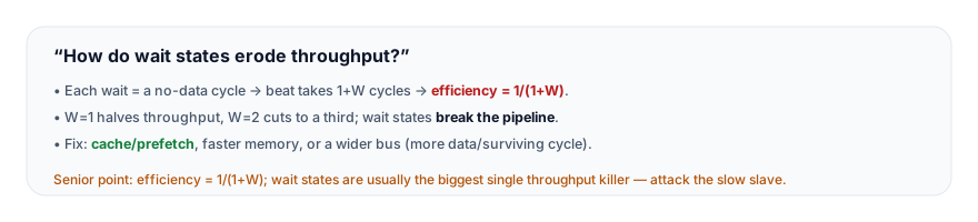
The answer that lands gives the formula and the unamortisable point: "Each wait state is a cycle where the slave holds HREADY low and no data moves. So a beat that takes W wait states occupies 1 + W cycles — one data cycle plus W wait cycles — and the per-beat efficiency is 1 over 1 plus W. That falls fast: one wait state halves throughput to 50%, two cut it to a third, four to a fifth. So a slow slave is often the dominant throughput loss — more than the address overhead or arbitration. The crucial point is that wait states are per-beat and can't be amortised by bursts. Bursts amortise the address-phase overhead — one address cycle over many beats — but every beat to a slow slave still pays its wait states, so a longer burst pays more total wait cycles, not fewer per beat. The efficiency stays capped at 1 over 1 plus W regardless of burst length. So if a slow slave is your bottleneck, bursting won't fix it — you have to reduce the wait states themselves: add a cache or prefetch buffer so the common-case access hits at full speed and the slow slave is touched only on a miss, use faster memory, or widen the bus to move more data per wait-stated beat. The classic example is a flash accelerator — a cache plus prefetch — that hides flash's wait states for code fetch. And because the penalty is so severe and common, a slow slave's wait states are usually the first thing to check in a throughput problem." The 1/(1+W) formula, the unamortisable-by-bursts insight, and the caching mitigation are the senior signals.

10. Practice Challenge

Compute and reason from the wait-state penalty.

1. The formula. Compute the per-beat efficiency for W = 0, 1, 3, and 7 wait states.
2. Unamortisable. Explain why a 16-beat burst to a 2-wait-state slave is still ~33% efficient.
3. Read the waveform. From Figure 2, explain why 1 wait state per beat gives 50% efficiency.
4. Diagnose. A slave gives 20% efficiency — how many wait states, and what's the fix?
5. Mitigate. Explain how caching hides the wait-state penalty and when it's the right fix.

11. Key Takeaways

• Each wait state is a no-data cycle — a beat with W wait states takes 1+W cycles, and per-beat efficiency = 1/(1+W) (W=1 → 50%, W=2 → 33%, W=4 → 20%).
• The penalty is reciprocal and severe — even one wait state halves throughput; a few devastate it.
• Wait states are per-beat and UNAMORTISABLE — bursts don't fix them (bursts amortise only the address overhead); every beat to a slow slave pays its wait states, capping efficiency at 1/(1+W) regardless of burst length.
• A slow slave is often the dominant throughput loss — usually the first thing to check in a throughput problem.
• Mitigate by reducing W or moving more per cycle — cache/prefetch (serve the common case at full speed — the memory hierarchy exists for this; e.g. a flash accelerator), faster memory (lower W), or a wider bus (more data per wait-stated beat).
• The memory hierarchy is fundamentally a wait-state-hiding structure — and data placement is budgeted against wait-state cost (hot data in fast memory).

12. What Comes Next

You now understand the wait-state penalty — the per-beat, unamortisable, reciprocal throughput loss from slow slaves. The next chapters quantify the other effects:

• Burst Efficiency (next) — how bursts amortise the address-phase overhead (the loss bursts do fix).
• Arbitration Overhead, Bridge Penalty, Bottleneck Analysis, Performance Debug — the remaining effects and how to debug performance.

To revisit wait states themselves, see Slave-Inserted Wait States; for the pipeline they break, see Pipelining Benefit.