Memory / Peripheral Bottlenecks

Chapters 14.1–14.7 quantified the individual performance effects; this chapter is the analysis method that uses them: bottleneck analysis — locating the slowest slave (or stage) in an AHB path. The governing principle (from chapter 13.8): achievable bandwidth is the minimum along the path — the slowest of the master's demand, the interconnect's capacity, and the slave's throughput. So to find the bottleneck, you trace the path and measure each stage, then identify the smallest — that's the bottleneck. Crucially, to find the bottleneck slave, you weight each slave's slowness by its access frequency: a frequently-accessed, moderately-slow slave can consume more total cycles than a rarely-used, very-slow one — so the frequent slow slave usually dominates, not the slowest-per-access. And after fixing the bottleneck, you re-measure — the bottleneck may have moved to the next-slowest stage. This chapter gives the bottleneck-analysis method: trace, measure, weight by frequency, fix the minimum, iterate.

1. What Is It?

Bottleneck analysis is the method of locating the slowest stage (usually a slave) that limits an AHB path's performance. The steps:

• Trace the path — follow a transfer's route: master → interconnect → slave (and back).
• Measure each stage — the master's demand, the interconnect/path capacity, each slave's throughput (set by its wait states).
• The bottleneck = the minimum — achievable bandwidth = min(master, path, slave); the smallest stage is the bottleneck.
• Weight slaves by frequency — the bottleneck slave is the one consuming the most cycles = slowness × access frequency (a frequent slow slave dominates).
• Fix and re-measure — fixing the minimum raises bandwidth; the bottleneck may then move to the next-slowest.

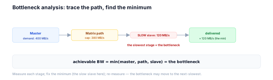
So bottleneck analysis is the systematic application of the "bandwidth = minimum along the path" principle (chapter 13.8) to find the limiting stage. It's not guessing — it's tracing and measuring: follow the transfer's path, quantify each stage's contribution (using chapters 14.1–14.7: wait states, bursts, arbitration, bridge), and identify the smallest. The smallest is the bottleneck — the only thing worth fixing (improving a non-bottleneck stage doesn't help). And the bottleneck slave specifically is found by weighting slowness by frequency — the slave that consumes the most cycles overall. So bottleneck analysis is the method to locate what's actually limiting performance, so you fix the right thing. So it's the find-the-minimum, weighted-by-frequency analysis method.

2. Why Does It Exist?

Bottleneck analysis exists because performance is set by the single slowest stage (the minimum along the path, chapter 13.8), so finding that stage is the prerequisite to improving performance — and because the naive approach (optimizing the slowest-per-access, or guessing) fails (it ignores access frequency and the minimum principle).

The minimum principle makes finding the bottleneck essential: achievable bandwidth = min along the path (chapter 13.8) — the slowest stage caps everything. So to improve performance, you must improve the slowest stage (the bottleneck) — improving any other stage does nothing (the minimum still caps). So you must first find the bottleneck (the minimum) — otherwise you might optimize the wrong stage (wasted effort). So bottleneck analysis exists because the minimum principle means only the bottleneck matters, so locating it is essential. So you find before you fix.

The weighting-by-frequency is why naive slowness-ranking fails: it's tempting to find the slowest-per-access slave and fix that. But the slowest slave might be rarely accessed — so it consumes few total cycles and isn't the bottleneck. Meanwhile a moderately-slow but frequently-accessed slave consumes many cycles and is the bottleneck. So the bottleneck slave is the one with the highest slowness × frequency (total cycles consumed), not the highest slowness alone. So bottleneck analysis must weight by frequency — and this is why a naive "find the slowest slave" approach can mislead. So the weighting exists to find the real bottleneck (cycle-consumption), not the apparent one (per-access slowness). So you weight by frequency.

The reason you re-measure after fixing is that the bottleneck moves: once you fix the slowest stage, it's no longer the slowest — some other stage is now the minimum (the new bottleneck). So fixing one bottleneck exposes the next. So bottleneck analysis is iterative: fix the minimum, re-measure, find the new minimum, fix it, repeat — until performance meets the goal (or further fixes have diminishing returns). So re-measuring exists because the bottleneck shifts. So bottleneck analysis exists because: performance is the minimum along the path, so only the bottleneck matters and finding it is essential (the why); the bottleneck slave is found by weighting slowness by frequency (not slowness alone — the method); and fixing it moves the bottleneck, so you iterate (the loop). So bottleneck analysis is the disciplined find-the-minimum, weighted-by-frequency, iterate method that ensures you optimize the right stage — the practical realization of the minimum principle. So this chapter gives the method that the earlier chapters' quantities feed into. (Chapter 14.9 adds the measurement tools to execute it.)

3. Mental Model

Model bottleneck analysis as finding the slowest step in an assembly line that's limiting output — the line's rate is set by its slowest station (the bottleneck), so you don't speed up the fast stations (no help — the slow one still caps output); you find the slowest station and speed it up; and crucially, "slowest" means most time spent overall, so a station that's a bit slow but handles every product matters more than one that's very slow but handles one rare product — and once you fix the bottleneck, a different station becomes the new slowest, so you re-check.

An assembly line (the AHB path) produces output (transfers/data) through a series of stations (stages: master, interconnect, slave). The line's output rate is set by its slowest station — the bottleneck (the minimum). If you speed up a fast station, the output doesn't improve — the slow station still caps it (you just have the fast station idle more, waiting). So to raise output, you must find and speed up the slowest station. Now, which station is the bottleneck? Not necessarily the one that's slowest per item — it's the one that consumes the most total time, which is slowness × how many items it handles. A station that's moderately slow but handles every product (high frequency) is a bigger bottleneck than one that's very slow but handles one rare product (low frequency). So you weight slowness by throughput-frequency. And once you fix the bottleneck station (speed it up), a different station is now the slowest — the bottleneck moved — so you re-check and fix the new one. You iterate until the line meets its target rate. So: find the slowest station (weighted by how much it's used), speed it up, re-check — don't waste effort on stations that aren't the bottleneck.

This captures bottleneck analysis: the assembly line = the AHB path; the stations = the stages (master, interconnect, slave); output rate set by the slowest station = bandwidth = minimum along the path; speeding up a fast station not helping = improving a non-bottleneck stage doesn't help; slowness × items handled = slowness × access frequency; the moderately-slow frequent station dominating = the frequent slow slave being the bottleneck; the bottleneck moving after a fix = re-measuring as the bottleneck shifts. Find the slowest weighted by use, fix it, re-check — don't optimize non-bottlenecks.

Watch a slow slave bottleneck a path:

The model's lesson: find the slowest station weighted by use, fix it, re-check — don't optimize non-bottlenecks. In the waveform, the slow slave sets the rate (every 4 cycles); the fast master/path can't help — only fixing the slave (the bottleneck) would.

4. Real Hardware Perspective

In hardware, bottleneck analysis is done with measurement: per-slave access counters, wait-state counters, and bus-utilization monitors reveal where the cycles go — and the analysis weights each slave's measured wait-cycle consumption by its access count.

The measurement instrumentation: to find the bottleneck, you measure (not guess). Hardware performance counters (or simulation/trace) capture: per-slave access counts (how often each slave is accessed), per-slave wait-state counts (how many wait cycles each slave inserts), bus utilization (active vs idle cycles), and grant-latency (arbitration waits). So in hardware, the analysis is data-driven — counters reveal where the cycles go. So measure first. (Chapter 14.9 details the tools.)

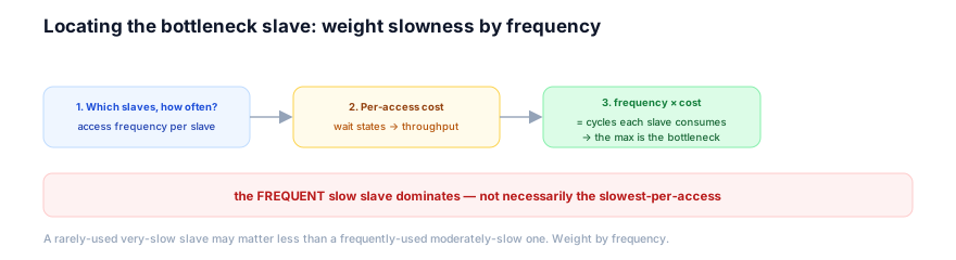
The weighting computation: with the measurements, you compute, per slave, the total cycles consumed = access count × per-access cost (≈ 1 + wait states). The slave with the highest total cycles is the bottleneck slave — it's where the most time is spent. This weights the per-access slowness by the frequency. So a slave accessed 1000× with 3 wait states (≈4000 cycles) is a bigger bottleneck than one accessed 10× with 10 wait states (≈110 cycles). So in hardware, you rank slaves by total cycles consumed (frequency × cost) to find the bottleneck. So compute the weighted cost.

The fix-and-re-measure loop: having found the bottleneck slave (most cycles), you fix it — typically by reducing its wait states (cache/prefetch, faster memory, chapter 14.4) or reducing its access frequency (algorithmic — fewer accesses). Then you re-measure — the bottleneck may have moved (now a different slave, or the arbitration, or the bridge consumes the most cycles). So you iterate. So in hardware, bottleneck analysis is: instrument (counters), measure (per-slave access counts + wait states + utilization), compute (frequency × cost per slave → the max is the bottleneck), fix (reduce the bottleneck's wait states or frequency), re-measure (iterate as the bottleneck moves). So the hardware method is data-driven, weighted-by-frequency, iterative. The quantities come from chapters 14.1–14.7 (wait states, bursts, arbitration, bridge); the method is this chapter; the tools are chapter 14.9. So the hardware reality: measure where the cycles go, fix the biggest consumer, repeat.

5. System Architecture Perspective

At the system level, bottleneck analysis is the core performance-engineering loop — it directs optimization effort to the one place that matters (the bottleneck), preventing wasted effort on non-bottlenecks, and it's iterative because fixing one bottleneck exposes the next.

The directing effort to the bottleneck: the most important system-level value is focus — bottleneck analysis tells you where to spend optimization effort: the bottleneck, and only the bottleneck. Because performance is the minimum along the path, only improving the minimum raises it — so optimizing anything else is wasted effort (it doesn't improve performance, and may add cost/complexity for no gain). So bottleneck analysis prevents wasted optimization — a common, costly mistake is optimizing a non-bottleneck (e.g. speeding up an already-fast stage, or adding bursts when the bottleneck is wait states) and seeing no improvement. So at the system level, bottleneck analysis is the focus mechanism — fix the right thing. So it's central to efficient performance work.

The iterative, moving-target nature: performance optimization is iterative because the bottleneck moves. You fix the current bottleneck (the slowest stage), and now a different stage is the slowest — the new bottleneck. So you re-measure and fix the new one. This continues until either performance meets the goal, or the remaining bottleneck is fundamental (e.g. the peak bandwidth, chapter 14.1) or uneconomical to fix. So at the system level, performance work is a loop: measure → find bottleneck → fix → re-measure → repeat. So you don't fix everything at once; you fix the current limiter, then the next. So it's iterative.

The diminishing returns and stopping: the iteration has diminishing returns — each fix moves the bottleneck, but eventually the remaining bottlenecks are small (the path is near-balanced) or hard (fundamental limits). So you stop when performance is good enough (meets the goal) or the cost of fixing the next bottleneck exceeds the benefit. So at the system level, bottleneck analysis is the iterative, focus-on-the-minimum performance loop — directing effort to the one limiting stage (preventing wasted optimization), iterating as the bottleneck moves, and stopping at the performance goal or diminishing returns. It's the performance-engineering discipline: don't optimize blindly; measure, find the bottleneck, fix it, repeat. The earlier chapters give the quantities (what each effect costs); bottleneck analysis gives the method (find the dominant cost); chapter 14.9 gives the tools (measure it). Together they're the AHB performance-engineering toolkit. So bottleneck analysis is the organizing method that makes the performance module actionable — turning the quantified effects into a procedure for actually improving a system.

6. Engineering Tradeoffs

Bottleneck analysis embodies the find-the-minimum, weight-by-frequency, iterate discipline.

• Fix the bottleneck vs optimize broadly. Fixing only the bottleneck (the minimum) raises performance with focused effort; optimizing broadly (non-bottlenecks too) wastes effort (no gain from non-bottlenecks). Focus on the bottleneck.
• Weight by frequency vs slowness alone. Ranking slaves by total cycles consumed (slowness × frequency) finds the real bottleneck; ranking by per-access slowness alone can mislead (a rare very-slow slave isn't the bottleneck). Weight by frequency.
• Iterate (re-measure) vs one-shot. Re-measuring after each fix catches the moved bottleneck; assuming the bottleneck is fixed (one-shot) misses the new limiter. Iterate until the goal.
• Measure vs guess. Measuring (counters, trace) reveals the actual bottleneck; guessing risks optimizing the wrong stage. Measure first (chapter 14.9).

The throughline: bottleneck analysis locates the slowest stage limiting an AHB path — achievable bandwidth = the minimum along the path (master, interconnect, slave), so trace the path, measure each stage, and find the smallest. The bottleneck slave is the one consuming the most cycles = slowness × access frequency (a frequent moderately-slow slave dominates a rare very-slow one). Only fixing the minimum raises performance (focus there); after fixing it, re-measure — the bottleneck moves to the next-slowest — and iterate until the goal or diminishing returns. It's the data-driven, weighted-by-frequency, iterative performance-engineering method that the earlier chapters' quantities feed into.

7. Industry Example

Perform bottleneck analysis on a slow system.

A system's throughput is below target; find and fix the bottleneck.

• Measure (instrument). Performance counters reveal: the CPU accesses flash (code) 60% of the time (with 3 wait states each), SRAM (data) 35% (zero-wait), and peripherals 5% (through the bridge). Bus utilization shows most cycles are wait states on flash.
• Weight by frequency. Compute cycles consumed: flash = 60% × ~4 cycles/access = dominant; SRAM = 35% × ~1 cycle = small; peripherals = 5% × ~5 cycles = small. So flash consumes the most cycles — it's the bottleneck (frequent and slow). (The peripherals are slowest-per-access but rare, so not the bottleneck.)
• Fix the bottleneck (flash). Add a flash accelerator (cache/prefetch, chapter 14.4) so the frequent code fetches hit fast (zero-wait), accessing slow flash only on a miss. The flash's effective wait states drop toward 0 — its cycle consumption plummets. Throughput jumps.
• Re-measure (bottleneck moved). After the flash fix, re-measure: now SRAM (35%, zero-wait) and the flash misses are small, but the peripheral accesses through the bridge or the arbitration might now be the largest remaining consumer — the bottleneck moved. Suppose arbitration (a DMA contending) is now the limiter.
• Fix the new bottleneck. Address the arbitration (e.g. move to a bus matrix so the CPU and DMA don't contend, chapter 14.6 / 13.3). Re-measure.
• Stop at the goal. Iterate until throughput meets the target. Eventually the remaining bottleneck is the peak bandwidth (chapter 14.1) or a fundamental limit — stop (further fixes have diminishing returns).

The example shows the method: measure (counters), weight by frequency (flash dominates — frequent and slow, not the rare-but-slowest peripheral), fix the bottleneck (cache the flash), re-measure (the bottleneck moved to arbitration), fix the new one, iterate to the goal. The key discipline: fix the frequent slow flash, not the rare slow peripheral — weighted by frequency. This is how bottleneck analysis is performed.

8. Common Mistakes

9. Interview Insight

Bottleneck analysis is a method interview topic — the minimum principle, the weight-by-frequency point, and the iterate-as-it-moves loop are the signals.

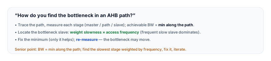
The answer that lands gives the principle, the weighting, and the loop: "Bottleneck analysis finds the slowest stage limiting an AHB path. The principle is that achievable bandwidth is the minimum along the path — the slowest of the master's demand, the interconnect's capacity, and the slave's throughput. So you trace the path and measure each stage, and the smallest is the bottleneck. Crucially, only the bottleneck matters: improving any other stage yields zero gain, because the minimum still caps the bandwidth. So you must measure to find it, not guess. To locate the bottleneck slave specifically, you weight each slave's slowness by its access frequency — the bottleneck is the slave consuming the most total cycles, which is per-access cost times access count. So a frequently-accessed moderately-slow slave, like code flash hit constantly, dominates a rarely-used very-slow slave, like an occasional peripheral. That's a key point: it's not the slowest-per-access slave, it's the one consuming the most cycles overall. Then you fix the bottleneck — for a slow flash, add a cache; for arbitration contention, use a matrix — and re-measure, because the bottleneck moves: once you fix the current one, a different stage is now the slowest. So it's iterative: measure, find the weighted minimum, fix it, re-measure, repeat, until you hit the target or the remaining bottleneck is fundamental." The minimum principle, the weight-by-frequency, and the iterate-as-it-moves loop are the senior signals.

10. Practice Challenge

Perform bottleneck analysis.

1. The principle. State why achievable bandwidth is the minimum along the path and what that implies for optimization.
2. Weight by frequency. Given two slaves (one slow+rare, one moderate+frequent), identify the bottleneck and explain why.
3. Read the waveform. From Figure 2, explain why the slow slave sets the rate and why fixing the master/path wouldn't help.
4. Iterate. Explain why you re-measure after fixing the bottleneck.
5. No-gain. Explain why optimizing a non-bottleneck stage yields zero improvement.

11. Key Takeaways

• Achievable bandwidth = the minimum along the path (master demand, interconnect capacity, slave throughput) — so the slowest stage is the bottleneck, and only fixing it raises performance.
• Trace the path and measure each stage — don't guess; use the earlier chapters' quantities (wait states, bursts, arbitration, bridge) and measurement tools (chapter 14.9).
• The bottleneck slave = slowness × access frequency — the slave consuming the most total cycles, not the slowest-per-access; a frequent moderately-slow slave dominates a rare very-slow one.
• Optimizing a non-bottleneck yields ZERO gain — the minimum still caps the bandwidth; fix only the bottleneck.
• Fix the minimum, then re-measure — the bottleneck moves to the next-slowest stage after a fix; performance work is iterative (measure → find → fix → re-measure → repeat).
• Stop at the goal or a fundamental limit — iterate while there are economical bottlenecks below the goal; stop at the target, the peak (chapter 14.1), or diminishing returns.

12. What Comes Next

You now have the bottleneck-analysis method — find the minimum (weighted by frequency), fix it, iterate. The final chapter provides the measurement tools and ties the whole module together:

• Performance Debug (next) — a method to measure and improve AHB performance, synthesizing all the effects (throughput, latency, wait states, bursts, arbitration, bridge) and the bottleneck-analysis loop into a practical debug procedure.

To revisit the minimum principle this builds on, see Bus Matrix Performance; for the dominant bottleneck cause, see Wait-State Penalty.