Bus Matrix Performance

This closes Module 13 by connecting the matrix's structure to its performance: how topology relates to achievable system bandwidth. The matrix's peak bandwidth scales with the number of slaves accessed concurrently (chapter 13.4) — but the achievable bandwidth is set by the bottleneck: the minimum along the path, not the matrix's peak. A master may demand high bandwidth, the matrix path may carry it, but if the target slave is slow or hot (shared by several masters), the slave caps throughput — likewise a shared link or an under-pipelined path can be the bottleneck. Topology is the cost-vs-bandwidth lever: a full crossbar (every master ↔ every slave) gives the most concurrency at the most area; a sparse matrix keeps the concurrency that matters at much lower area; a shared-link/partial topology cuts area further but creates contention points that cap bandwidth. The throughline: achievable bandwidth comes from matching the topology and the slave organization to the traffic pattern — spread traffic across slaves, bank hot memories, place data to hit different slaves. This chapter relates topology to bandwidth and gives the bottleneck-driven design approach.

1. What Is It?

Bus matrix performance is the achievable bandwidth a matrix delivers — determined by topology, slave organization, and traffic pattern, and capped by the bottleneck.

• Peak bandwidth — scales with the number of slaves accessed concurrently (up to N transfers/cycle for N busy slaves, chapter 13.4).
• Achievable bandwidth — the minimum along the path (the bottleneck): the slowest/hottest slave, a shared link, or an under-pipelined path caps throughput.
• Topology — full crossbar (max bandwidth, max area) vs sparse (near-full at lower area) vs shared-link (low area, capped bandwidth) — the cost-vs-bandwidth lever.
• Matching to traffic — the achievable bandwidth depends on how well the topology and slave organization fit the traffic pattern.

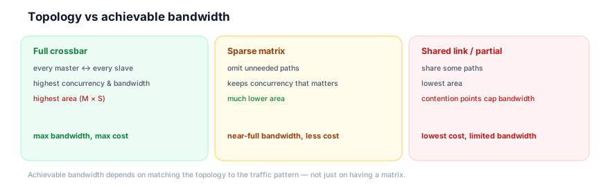
So bus matrix performance is not simply "the matrix is fast" — it's a function of peak (set by concurrency potential), bottlenecks (set by the slowest point along each path), topology (the cost/bandwidth structure), and traffic match (how well the design fits the actual access pattern). The matrix provides a peak bandwidth capability, but the delivered bandwidth is bottleneck-limited and traffic-dependent. So evaluating or designing for matrix performance means thinking about where the minimum is and whether the topology/organization fits the traffic — not just the matrix's theoretical peak. So bus matrix performance is the bottleneck-and-traffic-determined achievable bandwidth, shaped by topology and slave organization.

2. Why Does It Exist?

The bus matrix performance question exists because the matrix's peak capability (concurrency) is only realized when the whole path (master, matrix, slave) and the traffic pattern support it — so understanding what limits bandwidth (bottlenecks, topology, traffic) is essential to designing for the performance you actually need.

The peak vs achievable gap is the root: the matrix can carry N concurrent transfers (its peak, chapter 13.4) — but only if N slaves are actually being accessed by N masters and nothing along the paths limits them. In reality, the achievable bandwidth is less than peak because of bottlenecks: a slow slave (wait states) limits its path's throughput; a hot slave (multiple masters) serializes (chapter 13.3); a shared link (in a non-full topology) creates contention; an under-pipelined path may limit the clock. So there's a gap between the matrix's peak and what's achievable. So the performance question exists to understand and close that gap. So it's about realizing the peak, not just having it.

The bottleneck principle is the key insight: bandwidth along any path is the minimum of the bandwidths of the stages on that path (master demand, matrix path capacity, slave throughput). So the slowest stage — the bottleneck — sets the path's bandwidth, regardless of how fast the other stages are. A fast matrix can't help a slow slave; a fast slave can't help if a shared link throttles the path. So achievable bandwidth = the minimum along the path. So to raise bandwidth, you must find and fix the minimum (the bottleneck) — speeding up non-bottleneck stages does nothing. So the performance question exists to locate the bottleneck. So it's a min-finding problem.

The topology-and-traffic dependence is why design matters: the matrix's topology (full/sparse/shared-link) sets the path capacities and area — and the traffic pattern (which masters access which slaves, how often) determines which paths matter and where contention occurs. So the right topology and slave organization for a given traffic pattern maximizes achievable bandwidth per area — a full crossbar is wasteful if the traffic doesn't need all paths; a shared-link topology is fine if the shared paths aren't contended; spreading traffic across slaves (chapter 13.4) avoids hot-slave bottlenecks. So the performance question exists because the achievable bandwidth depends on matching the design (topology + slave organization) to the traffic — there's no one-size-fits-all. So bus matrix performance exists as a question because: the matrix's peak is only realized when the whole path and traffic support it (the peak-vs-achievable gap), the achievable bandwidth is set by the bottleneck (the minimum along the path — fix the min to improve), and it depends on matching topology and slave organization to the traffic pattern (no universal best). It's the design-for-performance lens on the matrix — turning the structural capability (concurrency) into delivered bandwidth by removing bottlenecks and fitting the traffic. So this chapter exists to teach how to get the matrix's bandwidth, not just that it has some.

3. Mental Model

Model bus matrix performance as a highway system's real throughput — building more lanes (a full crossbar) raises the peak capacity, but the actual traffic flow is limited by the worst bottleneck: a single-lane bridge (a slow slave), a popular exit everyone takes (a hot slave), or a shared on-ramp (a shared link); and the smart design isn't always "build maximum lanes everywhere" — it's matching the road capacity to where the traffic actually goes, and spreading destinations so they don't all funnel through one exit.

A highway system (the matrix) is built to move cars (transfers). Adding lanes (a full crossbar, more paths) raises the peak capacity — in theory, many cars flow in parallel. But the actual throughput is limited by the worst bottleneck along the routes people take: a single-lane bridge somewhere (a slow slave — every car crossing it is throttled), a popular exit that everyone takes (a hot slave — cars queue for the one exit regardless of how many highway lanes there are), or a shared on-ramp feeding multiple routes (a shared link — contention there caps the merged flow). So the highway's peak lane-count is irrelevant if there's a single-lane bridge on the route — the bridge sets the throughput (the minimum). And the smart design isn't "build maximum lanes everywhere" (wasteful — wide highways leading to a single-lane bridge help nothing); it's matching road capacity to where traffic actually goes (widen the bridge that's the bottleneck, not unused side roads) and spreading destinations (open multiple exits so cars don't all funnel through one — like spreading data across slaves). So real throughput comes from finding the bottleneck and fixing it, and fitting the roads to the traffic — not from maximum lanes alone.

This captures matrix performance: building lanes = topology (full crossbar = max lanes); peak capacity = the matrix's peak bandwidth; the single-lane bridge = a slow slave; the popular exit everyone takes = a hot slave; the shared on-ramp = a shared link/partial topology; the throughput limited by the worst bottleneck = achievable bandwidth = the minimum along the path; matching roads to traffic + spreading destinations = matching topology/slave organization to the traffic pattern (spread data, bank hot slaves). Real throughput is set by the bottleneck and the traffic fit — not the peak lane count.

Watch achievable bandwidth limited by a bottleneck slave:

The model's lesson: real throughput is set by the worst bottleneck, not the peak lane count. In the waveform, the CPU and matrix path could go every cycle, but the slow slave caps the path at one transfer per 3 cycles — the bottleneck sets the bandwidth.

4. Real Hardware Perspective

In hardware, matrix performance is shaped by the topology's path structure (full/sparse/shared), the slaves' throughput (wait states, banking), the matrix's pipelining (latency vs clock), and the address-map/data layout that determines traffic spread.

The topology's path structure sets the concurrency ceiling: a full crossbar instantiates a path (and per-slave arbiter) for every master-slave pair (M × S — chapter 13.3) — maximum concurrency, maximum area. A sparse matrix omits paths not needed by the traffic (e.g. the debug port reaches only memory) — fewer paths, less area, but the omitted paths can't carry traffic (fine if the traffic doesn't need them). A shared-link topology has multiple master-slave pairs share a physical path/arbiter — least area, but the shared path is a contention point (a bottleneck). So in hardware, topology directly sets the path structure and thus the concurrency ceiling and area. So topology is the first performance lever.

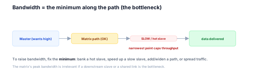
The slave throughput is often the real bottleneck: a slave's own speed (wait states, chapter 12.4) caps its path's bandwidth regardless of the matrix. A slow flash (many wait states) is a bottleneck; a hot slave (shared by masters, serialized — chapter 13.3) is a bottleneck. The hardware fix is at the slave: speed it up (caching/prefetch for flash), or bank it (split a hot memory into independently-arbitrated banks so accesses spread — chapter 13.4). So in hardware, slave throughput and banking are key performance levers — often more impactful than the matrix itself. So fix the slave bottleneck.

The pipelining and layout complete the picture: matrix pipelining (chapter 13.6) raises the clock (more bandwidth per second) at a latency cost — a performance lever for clock-limited matrices. And the address-map/data layout (chapter 13.4) determines traffic spread — placing each master's data in different slaves maximizes concurrent (parallel) access, while concentrating it creates hot-slave bottlenecks. So in hardware, the layout activates the matrix's concurrency. So in hardware, matrix performance is shaped by topology (path structure → concurrency ceiling/area), slave throughput (the common bottleneck → speed up or bank), pipelining (clock vs latency), and data layout (traffic spread → realized concurrency). The matrix's peak is set by topology, but the achievable bandwidth is set by the bottleneck among these — usually a slow/hot slave — and realized by a layout that spreads traffic. So the hardware performance is a whole-path, traffic-matched property.

5. System Architecture Perspective

At the system level, bus matrix performance is a co-design problem — the matrix topology, the memory/slave organization, the address map, and the data placement must be designed together for the expected traffic — and it's where the interconnect's value is actually delivered (or wasted).

The co-design requirement: the matrix's achievable bandwidth depends on multiple design decisions that must align: the topology (which paths exist), the slave organization (how many slaves/banks, their speeds), the address map (which addresses → which slaves), and the data placement (where each master's working set lives). These are interdependent — a full crossbar is wasted if data isn't spread across slaves; banking a memory only helps if the address map and placement route accesses to different banks; a sparse topology must include the paths the traffic actually uses. So matrix performance is a co-design of interconnect + memory + map + placement for the traffic. So at the system level, you don't design the matrix in isolation — you design the whole memory subsystem for the bandwidth goal. This is a key architectural discipline.

The traffic-pattern dependence makes it workload-specific: the right design depends on the expected traffic — which masters are active, what they access, how concurrently. A system where the CPU, DMA, and accelerator naturally hit different memories benefits hugely from a matrix (high concurrency); a system where they all hammer one shared buffer needs banking (to spread) or gets little benefit. So the architect must characterize the traffic (profile or model the access pattern) and design for it. So at the system level, matrix performance design is workload-driven — measure/estimate the traffic, then size the topology, organize the slaves, and place data to fit it. So it's not generic; it's traffic-specific.

The bottleneck-driven optimization is the method: since achievable bandwidth is the minimum along the path, improving performance means finding and fixing the bottleneck — and only the bottleneck (improving non-bottleneck stages wastes effort). So the optimization loop is: measure the achievable bandwidth, find the bottleneck (the slowest/hottest/most-contended stage), fix it (bank a hot slave, speed a slow one, add a path, spread traffic), re-measure (the bottleneck may have moved), repeat. So matrix-performance tuning is iterative bottleneck-removal. So at the system level, bus matrix performance is a co-design problem (interconnect + memory + map + placement, designed together for the traffic), workload-driven (characterize the traffic, design for it), and optimized by iterative bottleneck-removal (find and fix the minimum). The matrix provides the concurrency capability, but delivering bandwidth requires designing the whole subsystem for the actual workload and removing bottlenecks. This is where the interconnect module's understanding (multiple masters, multiple slaves, matrix, parallel access, decode+arbitrate, routing, HREADY) culminates: in designing a matrix-based memory subsystem that delivers the bandwidth the system needs — a capstone systems-design skill. So matrix performance is the practical payoff of the whole module.

6. Engineering Tradeoffs

Bus matrix performance embodies the topology-vs-cost, bottleneck-limited, traffic-matched design.

• Full crossbar vs sparse vs shared-link. Full crossbar: max concurrency/bandwidth, max area. Sparse: keeps the concurrency that matters, much less area (omit unused paths). Shared-link: least area, but shared paths cap bandwidth (contention). Choose per the traffic's path needs.
• Slave speed/banking vs matrix improvement. Often the slave is the bottleneck — speeding it up (caching) or banking it (spread access) helps more than improving the matrix. Fix the actual bottleneck, not the matrix peak.
• Pipelining: clock vs latency. Pipelining the matrix raises the clock (more bandwidth/second) at a latency cost (chapter 13.6). Worth it for clock-limited, throughput-oriented systems; avoid for latency-critical ones.
• Design-for-traffic vs generic. Matching the topology/slave-organization/placement to the expected traffic maximizes achievable bandwidth per area; a generic max-everything design wastes area, and a mismatched design wastes the matrix (hot-slave bottleneck). Co-design for the workload.

The throughline: the matrix's peak bandwidth scales with concurrently-accessed slaves, but the achievable bandwidth is the minimum along the path (the bottleneck — slow/hot slave, shared link, under-pipelined path), not the peak. Topology (full crossbar / sparse / shared-link) trades cost for bandwidth. Real performance comes from matching the topology AND slave organization AND data placement to the traffic pattern — spread traffic across slaves, bank hot memories — and from iterative bottleneck-removal (find and fix the minimum). It's a co-design, workload-driven problem: the matrix provides the concurrency capability; delivering bandwidth requires designing the whole memory subsystem for the actual traffic.

7. Industry Example

Tune a matrix-based system for bandwidth.

A system has a CPU, a DMA, and a video accelerator, needing high aggregate memory bandwidth.

• Naive design (hot slave). Initially, all three masters share one large SRAM via a matrix. Measured bandwidth is low — barely better than a shared bus. Why? The single SRAM is a hot slave: all three masters contend for it, and its arbiter serializes them. The matrix's paths are idle of concurrency because the traffic funnels to one slave. The matrix didn't help.
• Find the bottleneck. Profiling shows the SRAM is the bottleneck (100% contended). The matrix and masters could go faster, but the single SRAM caps throughput — the minimum along the path.
• Fix: bank the memory. The architect banks the SRAM into four independently-arbitrated banks and places each master's working set (and interleaves shared data) so the masters predominantly hit different banks. Now the masters access different slaves (banks) concurrently — the matrix's parallel access (chapter 13.4) is activated. Bandwidth jumps toward the peak.
• Match the topology. The debug port (a fourth master) only needs occasional memory access — so its paths to the video buffer are omitted (sparse matrix), saving area without hurting bandwidth (debug doesn't need video-buffer bandwidth).
• Address a slow slave. Flash (holding code) is slow (wait states) — a bottleneck for the CPU's fetches. The fix: a flash cache/prefetch (speeding the common-case fetch), reducing that bottleneck.
• Pipeline for clock. The matrix is pipelined (chapter 13.6) to hit the target clock (more bandwidth/second), accepting a cycle of latency — acceptable for the throughput-oriented video workload.
• Re-measure. After banking, sparsifying, caching flash, and pipelining, the achievable bandwidth approaches the aggregate demand — the bottleneck removed, the layout matched to the traffic. The matrix now delivers.

The example shows the bottleneck-driven, traffic-matched design: the naive single-SRAM design wasted the matrix (hot slave); banking spread the traffic (activating concurrency); sparse topology saved area; flash caching and pipelining removed other bottlenecks. The matrix delivered bandwidth only after the whole subsystem was co-designed for the traffic and the bottleneck removed. This is how matrix performance is achieved in practice.

8. Common Mistakes

9. Interview Insight

Bus matrix performance is a systems interview topic — the peak-vs-achievable distinction, the bottleneck principle, and the co-design-for-traffic approach are the signals.

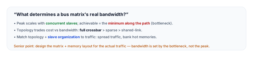
The answer that lands gives the bottleneck principle and the co-design approach: "A bus matrix's peak bandwidth scales with the number of slaves accessed concurrently — up to N transfers per cycle. But the achievable bandwidth is set by the bottleneck: the minimum along the path, not the peak. A master might demand high bandwidth and the matrix path might carry it, but if the target slave is slow (wait states) or hot (shared by multiple masters, so its arbiter serializes them), the slave caps the throughput — likewise a shared link in a non-full topology, or an under-pipelined path. So bandwidth is the minimum of the master demand, the path capacity, and the slave throughput. Topology is the cost-versus-bandwidth lever: a full crossbar gives maximum concurrency at maximum area; a sparse matrix keeps the concurrency that matters at much lower area by omitting unused paths; a shared-link topology cuts area but caps bandwidth at contention points. The crucial point is that a matrix doesn't guarantee bandwidth — you have to match the topology and the slave organization and the data placement to the traffic pattern: spread each master's working set across different slaves, bank hot memories so accesses hit different banks, and include the paths the traffic actually uses. And you optimize by finding and fixing the bottleneck — only the minimum matters — then re-measuring, since the bottleneck may move. So it's a co-design problem: the matrix provides the concurrency capability, but delivering bandwidth requires designing the whole memory subsystem for the actual workload." The peak-vs-achievable distinction, the bottleneck principle, and the co-design-for-traffic approach are the senior signals.

10. Practice Challenge

Reason from bus matrix performance.

1. Peak vs achievable. Explain the difference and why achievable is set by the bottleneck.
2. The bottleneck principle. Explain why bandwidth is the minimum along the path and why only fixing the bottleneck helps.
3. Read the waveform. From Figure 2, explain why the slow slave caps the path's bandwidth despite the fast master and path.
4. Topology. Compare full crossbar, sparse, and shared-link on cost and bandwidth.
5. Co-design. Describe how you'd design a matrix subsystem to deliver bandwidth for a given traffic pattern.

11. Key Takeaways

• Peak vs achievable: the matrix's peak bandwidth scales with concurrently-accessed slaves, but the achievable bandwidth is the minimum along the path (the bottleneck), not the peak.
• The bottleneck principle: bandwidth = min(master demand, path capacity, slave throughput); the slowest stage caps it, and only fixing the bottleneck raises it.
• Common bottlenecks: a slow slave (wait states), a hot slave (shared → serialized), a shared link (contention), an under-pipelined path (clock-limited).
• Topology trades cost for bandwidth: full crossbar (max bandwidth/area) > sparse (near-full at less area, omit unused paths) > shared-link (least area, capped bandwidth).
• A matrix doesn't guarantee bandwidth — you must match the topology, slave organization, and data placement to the traffic pattern (spread traffic across slaves, bank hot memories) to realize the concurrency.
• It's a co-design, bottleneck-removal problem — design the whole memory subsystem for the actual workload, then iteratively find and fix the bottleneck (it may move). The capstone of the interconnect module: turning structural concurrency into delivered bandwidth.

12. What Comes Next

This completes Module 13 — AHB Bus Matrix & Interconnect. You now understand multiple masters, multiple slaves, the bus matrix concept, parallel slave access, the decoder+arbiter combination, interconnect routing, HREADY aggregation, and bus matrix performance — the full picture of how AHB scales to a concurrent multi-master fabric and how to design it for bandwidth. The next module turns to system-level performance more broadly:

• Module 14 — Performance (coming next) — turning the protocol into bandwidth and finding why a real system is slow: bandwidth, latency, outstanding depth, burst efficiency, and bottleneck analysis.

To revisit the matrix mechanics this performance view builds on, see The Bus Matrix Concept, Parallel Slave Access, and Interconnect Routing.