Address Phase Leads Data Phase

This chapter pins down the single most quantitative fact of AHB timing: the address phase leads its own data phase by exactly one cycle. Chapter 5.1 established the two-phase structure; here we make the offset precise. For each transfer, the address is on cycle N and its data is on cycle N+1 — a fixed one-cycle lead. We show why the offset is exactly one cycle, what the lead is for, and — importantly — how the lead is preserved when a wait state stretches the data phase. This precision is what lets you read a waveform exactly and associate each data beat with the right address.

1. What Is It?

The rule is exact: a transfer's data phase is the cycle immediately after its address phase. If beat N's address is driven in cycle N, beat N's data moves in cycle N+1 — a one-cycle lead of address over data.

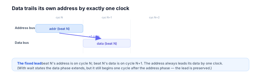
Two consequences of the exact offset:

• To find a beat's data, look one cycle after its address. The data for the address on cycle N is on cycle N+1 — read diagonally (chapter 5.1).
• The next transfer's address overlaps this transfer's data. Because address leads data by one, in cycle N+1 you see beat N's data and beat N+1's address — the overlap.

The lead is exactly one cycle in the no-wait-state case. When a subordinate inserts wait states, the data phase extends (it takes more cycles to complete), but it still begins one cycle after the address phase — so the lead between an address and the start of its data is preserved; the data phase just stretches.

2. Why Does It Exist?

The lead is exactly one cycle because that is precisely the time a synchronous register stage takes — and one register stage is exactly what AHB needs for decode without over-padding the latency.

The address-phase information is registered at the clock edge and used the next cycle (chapter 5.1). A single register introduces exactly one cycle of delay — so the data, which acts on the registered address, is exactly one cycle behind. The offset is one cycle because there is one register stage between presenting the address and moving the data. Could it be more? A deeper pipeline (more register stages) would push the data further behind the address, adding latency for no benefit on a bus that only needs one cycle to decode. Could it be zero? Same-cycle address and data would leave no time to decode the address and select the subordinate (chapter 2.3). So one cycle is the minimum offset that allows decode, and AHB uses exactly that minimum — no more.

The lead exists at all (as opposed to a single-cycle, no-pipeline transfer) for the two reasons from Module 2, now seen as the purpose of the one-cycle offset:

• Decode time. During the address-phase cycle, the decoder resolves the selection and the subordinate prepares. The one-cycle lead is exactly this preparation window. Without it, the data phase would arrive before the subordinate knew it was the target.
• Overlap (throughput). Because the address leads the data by one cycle, the next transfer's address phase falls in the same cycle as the current transfer's data phase — the overlap that gives one transfer per cycle. The lead is what creates the overlap; without an offset, there would be nothing to overlap.

So the one-cycle lead exists, and is exactly one cycle, because: a single register stage is the minimum needed to give the decoder and subordinate their setup cycle, and that same one-cycle offset is what enables the throughput-giving overlap. One register, one cycle of lead, two payoffs — and no more cycles than necessary, keeping the per-transfer latency minimal.

3. Mental Model

Model the lead as a kitchen where the order is called one beat before the dish is plated.

The waiter calls an order (the address phase) — "table 4, the salmon." One beat later, the kitchen plates that dish (the data phase). The dish is always one beat behind its order — exactly one, because the kitchen needs that one beat to grab the right ingredients (decode and prepare). The waiter does not wait for the dish before calling the next order; they call the next order (table 5) in the same beat the kitchen plates table 4's — the overlap. So at any beat, an order is being called and the previous order's dish is being plated, one beat apart.

If the kitchen is slow on one dish (a wait state), it takes extra beats to plate it, and the waiter holds the next order until the slow dish is out — the lead between each order and its own dish is preserved (still one beat from call to start-of-plating), but the line pauses while the slow dish finishes.

Watch the exact one-cycle lead, including a wait state:

The model's lesson: the dish is plated exactly one beat after its order is called — the one-cycle lead — and a slow dish stretches its plating (a wait state) while the next order is held, preserving the lead. In the waveform, address A on T0 leads its data; the wait state at T1 extends data A and holds address B, but the address-to-data-start lead stays one cycle.

4. Real Hardware Perspective

In hardware, the one-cycle lead is the latency of the address register, and the wait-state interaction is about extending the data phase while preserving the lead.

The master drives the address-phase signals in cycle N; they are registered at the clock edge and the data movement acts on them in cycle N+1. The one-cycle lead is exactly this register's latency — there is no additional delay because there is only one register stage. So in hardware, "address leads data by one cycle" is simply "the address is registered once before the data phase uses it." The minimality (one stage) is deliberate: it gives decode time without adding latency.

The wait-state interaction is the precise part. A wait state (HREADY low, chapter 3.8) does not change the lead between an address and the start of its data phase — that is still one cycle. What it does is extend the data phase: the data phase, which began one cycle after the address, now takes more than one cycle to complete because HREADY is held low. Meanwhile, the next transfer's address phase — which would normally follow immediately — is held until the current data phase completes (the master holds its address-phase outputs, chapter 2.3). So the pipeline pauses: the current data phase stretches, the next address waits, but the fundamental "address leads its own data by one cycle" relationship is intact. The lead is between an address and the beginning of its data; the wait state stretches the end of the data.

This distinction — lead preserved, data phase extended — is the key hardware reading skill for stalled transfers. On a capture with wait states, you still associate each data beat with the address one cycle before it started; the wait state just means the data beat occupies multiple cycles (held until HREADY high) and the next address is delayed. A common error is to think a wait state changes the address-to-data offset; it does not — it extends the data phase's duration and holds the next address, but the one-cycle lead from address to data-start is invariant.

So in hardware, the one-cycle lead is the address register's single-stage latency, invariant under wait states; what wait states change is the duration of the data phase and the timing of the next address, not the lead itself. Reading this correctly — lead fixed, data phase stretchable — is essential for analyzing real, stalled transfers.

5. System Architecture Perspective

At the system level, the fixed one-cycle lead is what makes AHB timing predictable and analyzable — every master and subordinate is designed to it, and timing tools rely on it.

Because the lead is fixed at one cycle, every component knows exactly when data will follow an address: a subordinate knows its data phase is the cycle after the address it sampled; a master knows its data will be expected one cycle after it drives the address. This fixed relationship is part of the timing contract (chapter 5.1) — components interoperate because all agree on the one-cycle lead. A subordinate from one vendor and a master from another work together because both implement "data one cycle after address." So the fixed lead is a cornerstone of AHB's composability: it is a precise, shared timing assumption.

The fixed lead also makes timing analysis and verification tractable. A protocol checker can assert the exact relationship: every data beat must correspond to the address one cycle before its start; a data phase must not appear without its address having led it by one cycle. Deviations (data without a preceding address, or a wrong offset) are flagged as timing violations. So the fixed lead is a checkable property — verification encodes "address leads data by one cycle," and the wait-state behaviour ("data phase extends, lead preserved") is checked too. This makes timing correctness a precise, automatable property rather than a judgement call.

For performance, the fixed lead is the basis of the one-transfer-per-cycle ceiling (chapter 5.1): because the address leads the data by exactly one cycle, the overlap is exactly one transfer per cycle when the pipe is full. Wait states (which extend the data phase) are the deviations below this ceiling — and because the lead is fixed, you can precisely attribute lost cycles to the extended data phases (wait states) versus other bubbles. So the fixed lead underpins both the throughput ceiling and the precise accounting of deviations from it. This precision — a known, fixed timing relationship — is what makes AHB timing engineering systematic rather than ad hoc.

So at the system level, the fixed one-cycle lead is a shared timing contract (composability), a checkable property (verification), and the basis of precise performance accounting — the quantitative backbone of AHB timing.

6. Engineering Tradeoffs

The one-cycle lead reflects the minimal-offset choice.

• One-cycle offset vs deeper. One register stage (one-cycle lead) is the minimum that gives decode time, and AHB uses exactly that. A deeper pipeline could permit a higher clock but adds per-transfer latency and more hazards (more stages between address and data). For AHB's target (moderate frequency, simplicity), the shallow one-cycle offset is the right balance — minimal latency, enough decode time.
• Fixed lead vs variable. Making the lead fixed at one cycle (rather than variable) keeps timing predictable, checkable, and interoperable, at the cost of no flexibility in the offset. Variable offsets would complicate every component and break the simple timing contract. AHB chooses the fixed offset; flexibility where needed (for slow subordinates) is provided by extending the data phase (wait states), not by varying the lead.
• Extend-the-data-phase (wait states) vs change-the-lead. Accommodating slow subordinates by extending the data phase — while keeping the lead fixed — preserves the predictable address-to-data relationship. The alternative (varying the address-to-data offset per subordinate) would destroy predictability. So AHB absorbs subordinate speed variation in the data phase's duration, not the lead, keeping the offset invariant.
• Latency vs throughput (restated). The one-cycle lead is a one-cycle latency per transfer that streams hide but isolated accesses pay (chapter 5.1). Keeping it to exactly one cycle minimizes that latency while still enabling the overlap. A larger lead would worsen isolated-access latency for no throughput gain.

The throughline: AHB uses the minimal fixed one-cycle lead — exactly the register latency needed for decode — and absorbs all timing variation in the data phase's duration (wait states), keeping the address-to-data offset invariant. This minimality and fixedness are what make AHB timing low-latency, predictable, and checkable.

7. Industry Example

Trace the one-cycle lead through a stream with a wait state.

A processor reads a run of words, one of which hits a slow subordinate.

• The fixed lead in a clean stream. The processor drives address A in cycle 1; data A returns in cycle 2 (one-cycle lead). Address B in cycle 2; data B in cycle 3. Address C in cycle 3; data C in cycle 4. Each data beat is exactly one cycle after its address — the fixed lead, with the overlap giving one transfer per cycle.
• A wait state on one beat. Suppose the subordinate for beat B is slow and inserts a wait state. Address B is driven in cycle 2 (one cycle after... well, in the overlapped stream). Data B's phase begins in cycle 3 (one-cycle lead, preserved) but the subordinate holds HREADY low, so data B does not complete until cycle 4 — the data phase is extended by one cycle. Meanwhile address C is held (not advanced) until data B completes. So the pipeline pauses for the wait cycle.
• Reading the capture correctly. On the stalled capture, the engineer still associates data B with address B (one cycle before data B's start), and reads the wait state as extending data B's phase and delaying address C — not as changing the address-to-data offset. The lead from address B to data-B-start is still one cycle; the wait state is a stretch of data B's duration. Mis-reading this (thinking the offset changed) would mis-associate the beats.
• The performance accounting. The clean beats run at one per cycle (the ceiling, from the fixed lead). The wait state is one cycle below the ceiling — precisely attributable because the lead is fixed: a known one-cycle lead means the only deviation is the extended data phase (the wait state). So the throughput loss is exactly the wait cycle, cleanly accounted.

The stream shows the fixed lead delivering one-per-cycle throughput, and the wait state extending a data phase while preserving the lead — read correctly by associating each data beat with the address one cycle before its start. This precise reading is what the chapter trains.

8. Common Mistakes

9. Interview Insight

This tests the precise offset and the wait-state subtlety.

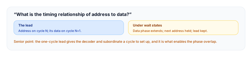
The answer that lands gives the exact offset and the wait-state behaviour: "The address phase leads its own data phase by exactly one cycle — beat N's address is on cycle N, its data on cycle N+1 — because the address is registered once before the data phase uses it, which is the minimum needed to decode and select the subordinate. Under wait states, the data phase extends (HREADY low holds the beat) and the next transfer's address is held, but the one-cycle lead from an address to the start of its data is preserved — the wait state stretches the data phase's duration, not the offset." The exact-one-cycle offset and the lead-preserved-under-wait-states point are the senior signals.

10. Practice Challenge

Reason from the exact offset and the wait-state behaviour.

1. State the offset. Give the exact lead of address over data and why it is that value.
2. Read the lead. From Figure 1, identify which cycle holds beat N's address and which holds its data.
3. Handle a wait state. From Figure 2, explain what the wait state does to the data phase and the next address, and what it does not do to the lead.
4. Associate beats. On a stalled capture, describe the rule for matching each data beat to its address.
5. Catch the error. A colleague says a wait state increased the address-to-data offset. Correct them.

11. Key Takeaways

• The address phase leads its own data phase by exactly one cycle — beat N's address on cycle N, its data on cycle N+1.
• The offset is one cycle because of one register stage — the minimum needed for decode; not zero (no decode time), not more (needless latency).
• The lead serves decode time and the overlap — the address-phase cycle is the subordinate's setup window, and the one-cycle offset is what makes the phase overlap (one transfer/cycle) possible.
• Wait states extend the data phase and hold the next address, but preserve the lead — beat N's data phase still begins on cycle N+1; the wait stretches its duration.
• Associate each data beat with the address one cycle before its start — the correct reading of stalled captures; the lead is fixed, the data-phase duration is stretchable.
• The fixed lead is a timing contract and a checkable property — it underpins composability, verification, and the precise accounting of throughput and its deviations.

12. What Comes Next

You now have the exact address-to-data offset. The next chapter uses it to align the control signals with the right data:

• 5.3 — Control / Data Alignment (coming next) — how the address-phase control governs the data that moves in the following data phase, and the alignment confusion to avoid.
• 5.4 — Read Transfer Timing (coming soon) — a read walked cycle by cycle through both phases.

To revisit the pipeline structure this offset belongs to, see The Two-Phase Pipeline; for the wait states that extend the data phase, see HREADY & HREADYOUT and The Data Phase. For the broader protocol map, see the AMBA family overview.